Llama is Meta AI’s large language model (LLM), with variants ranging from 7 billion to 70 billion parameters. Llama uses a transformers-based decoder-only model architecture, which specializes at language token generation. To train a model from scratch, a dataset containing trillions of tokens is required. The Llama family is one of the most popular LLMs. However, training Llama models can be technically challenging, prolonged, and costly.
In this post, we show you how to accelerate the full pre-training of LLM models by scaling up to 128 trn1.32xlarge nodes, using a Llama 2-7B model as an example. We share best practices for training LLMs on AWS Trainium, scaling the training on a cluster with over 100 nodes, improving efficiency of recovery from system and hardware failures, improving training stability, and achieving convergence. We demonstrate that the quality of Llama 2-7B trained on Trainium is of comparable quality to the open source version on multiple tasks, ranging from multi-task language understanding, math reasoning, to code generation. We also demonstrate the scaling benefits of Trainium.
What makes distributed training across over 100 nodes so challenging?
Training large-scale LLMs requires distributed training across over 100 nodes, and getting elastic access to large clusters of high-performance compute is difficult. Even if you manage to get the required accelerated compute capacity, it’s challenging to manage a cluster of over 100 nodes, maintain hardware stability, and achieve model training stability and convergence. Let’s look at these challenges one by one and how we address them with Trainium clusters during the end-to-end training:
- Distributed training infrastructure efficiency and scalability – Training LLMs is both computation and memory intensive. In this post, we show you how to enable the different parallel training algorithms on Trainium and select the best hyperparameters to achieve the highest throughput of Llama 2-7B on the Trainium cluster. We also demonstrate the implementations of other memory and computation optimization techniques such as coalescing layers and data type selection on Trainium. Empirically, we have proven that Trainium clusters can reduce costs by up to 46% compared to comparable Amazon Elastic Compute Cloud (Amazon EC2) instances.
- Efficient hardware and system recovery – End-to-end LLM training at this scale will inevitably encounter hardware or system failures. We demonstrate how to efficiently enable checkpoint saving and automatically recover using the NeuronX Distributed library. Empirically, we demonstrate that with automatic failure recovery, the effective utilization of hardware computing hours reaches 98.81% compared to 77.83% with a manual recovery method.
- Training stability and convergence – Finally, frequent occurrence of spikes of loss functions in pre-training deep neural networks such as Llama 2 can lead to catastrophic divergence. Due to the large computation cost required for training LLMs, we want to reduce loss function spikes, improve training stability, and achieve convergence of training. We demonstrate best practices and implementation of techniques such as scaled initialization, gradient clipping, and cache management on Trainium clusters to achieve this. We also show how to monitor and debug for training stability.
Llama 2-7B pre-training setup
In this section, we discuss the steps for setting up Llama 2-7B pre-training.
Infrastructure
Setting up the Llama 2-7B infrastructure consists of the following components:
- EC2 cluster – The training cluster includes 128 trn1.32xlarge instances (nodes), totaling 2048 Trainium accelerators. The networking among the instances is connected through 8×100 Gbps EFAs. We mounted 56 TB Amazon FSx storage for immediate data storage and checkpoint saving and loading. The raw training data was saved on Amazon Simple Storage Service (Amazon S3) buckets.
- Orchestration – We first trained the Llama 2-7B from scratch using a trn1.32xlarge cluster that is managed through Amazon Elastic Kubernetes Service (Amazon EKS). For details about the setup procedure, refer to Train Llama2 with AWS Trainium on Amazon EKS. We followed the same procedure but set up the cluster at a much larger scale with 128 trn1.32xlarge instances.
- Container build – We used a customer Docker image that was built based on the following training containers and included the Llama 2-7B training source files. We stored the customer Docker image in an Amazon Elastic Container Registry (Amazon ECR) registry and deployed it in EKS pods. The following diagram shows the architecture of the cluster and container setup.
Data preparation
The original format of the training dataset contains a large number of compressed files. To use this dataset, we first converted them into a format compatible with the Hugging Face dataset package. We used the Apache Arrow format (the default storage format for datasets) to combine all data into a single file and a single block of a file. This method significantly reduces load times for TB-sized datasets compared to the default method of loading many separate files.
We first downloaded the preprocessed training dataset, a small subset of the full dataset that contains 12 trillion tokens, using a special EC2 instance with 20–30 TB of memory. The data download script is as follows:
The dataset is processed for optimized storage and access:
    import pyarrow as pa
    import time

    a = time.time()
    stream = pa.memory_map("~/<data path>/arrow/train.arrow")
    stream = pa.ipc.open_stream(stream)
    table = stream.read_all()
    print("completed step 1 in seconds: ", time.time() - a)

    ca = table["text"]
    l = ca.to_pylist()
    schema = pa.schema({"text": pa.large_string()})
    arr = pa.array(l, type=pa.large_string())

    with pa.OSFile("~/<data path>/arrow/train.arrow", "wb") as sink:
        with pa.ipc.new_stream(sink, schema=schema) as writer:
            batch = pa.record_batch([arr], schema=schema)
            writer.write(batch)
    print("completed step 2 in seconds: ", time.time() - a)
On the same instance, we cleaned up the dataset and uploaded the clean dataset to an S3 bucket. We then used a 128 trn1.32xlarge cluster to perform tokenization and packaging (such as dynamically filling sequences and applying masking mechanisms) online during training. Compared with offline packaging methods, this online method saves tremendous development time and computing resources, especially for multiple experiments that use different large datasets and tokenizers.
Model hyperparameters
We adopted the same training hyperparameters as Llama models. Specifically, we used a cosine learning rate scheduler with the same maximum learning rate of 3𝑒−4 and the same minimum learning rate of 3𝑒−5. We followed the same linear warmup of 2,000 steps. The following figure shows a plot of the overall learning rate scheduler.

We used the AdamW optimizer with 𝛽1 = 0.9 and 𝛽2 = 0.95. We used weight decay value of 0.1 for all parameters, including normalization weights. For training stability, gradient-norm clipping of 1.0 was applied. For a different model setup, such as Llama 3, these parameters need to be tuned for optimal performance.
Distributed training infrastructure efficiency and scalability
During the training, we applied general optimization techniques, such as activation checkpointing, model and data parallelism, and computation and communication overlapping in Trainium through the Neuron SDK, as well as some unique enhancement such as BF16 with stochastic rounding. In this section, we list the key features and configurations used in our model pre-training to improve training efficiency.
Model and data parallelism
Neuron supports tensor parallelism (TP), pipeline parallelism (PP), sequence parallelism (SP), and data parallelism (DP). For the 7B model with 4,096 sequence length, we found that a TP degree of 8, PP degree of 1, SP degree of 8, and DP degree of 512 yields the highest training throughput. On a trn1.32xlarge instance cluster, this leads to having four model copies per instance.
We used a global batch size of 1,024 sequences with a maximum sequence length of 4,096 tokens. Each step covered about 4 million tokens. The gradient accumulation step is 2, which resulted in the actual batch size per Neuron core being 1. The following figure illustrates the data parallelism and tensor parallelism we applied in the training.

Neuron Distributed library
AWS Neuron is the SDK used to run deep learning workloads on AWS Inferentia and Trainium-based instances. It includes the compiler, runtime, and profiling tools. It supports a variety of data types, including FP32, BF16, FP16, and stochastic rounding. The Neuron SDK enables tensor parallelism, pipeline parallelism, and data parallelism distributed strategies through the NeuronX Distributed library. This allows trade-offs between preserving the high accuracy of trained models and training efficiency in throughput and memory consumption. We applied the following features in the training process:
- Selective activation checkpointing – We used selective activation checkpointing to improve training efficiency. It has a slightly higher memory cost than full activation checkpointing, but increases the overall training throughput.
- BF16 with stochastic rounding – We compared three precision settings: BF16, BF16 with SR, and mixed precision training. Empirically, we found that BF16 with SR showed the same convergence behavior as mixed precision training, with higher training throughput and lower memory footprint; whereas the training loss of BF16 diverged. Therefore, we chose BF16 with SR in our pre-training exercise.
- Coalescing layers with the same inputs – We coalesced linear layers with the same inputs to reduce the communication in tensor and sequence parallelism, and improve the efficiency of matrix operations. Specifically, the Q, K, and V layers in an attention block are coalesced, and the two linear projections layers in SwiGLU are also coalesced. This optimization technique is generic to LLMs. The following are the example code snippets:
q_proj, k_proj, v_proj were merged into qkv_proj
gate_proj, up_proj were merged into gate_up_proj
- Compiler optimization – We used the compiling flag
--distribution-strategy=llm-trainingto enable the compiler to perform optimizations applicable to LLM training runs that shard parameters, gradients, and optimizer states across data parallel workers. We also used--model-type=transformer, which performs optimizations specific to transformer models. We set the Neuron environment variableNEURON_FUSE_SOFTMAX=1to enable compiler optimizations on custom lowering for Softmax operation. Finally, we usedNEURON_RT_ASYNC_EXEC_MAX_INFLIGHT_REQUESTS=3to reduce training latency with asynchronous runs. This overlaps some runs of accelerators and host (CPU).
The following table summarizes all hyperparameters used in our pre-training exercise.
| . | . | Trn – NxD |
| Optimization parameters | Seq_len | 4096 |
| . | Precision | bf16 |
| . | GBS | 1024 |
| . | learning rate | 3.00E-04 |
| . | min_lr | 3.00E-05 |
| . | weight decay | 0.1 |
| . | grad_clip | 1 |
| . | LR scheduler | cosine |
| . | warmup step | 2000 |
| . | constant step | 0 |
| . | AdamW (bete1, beta2) | (0.9, 0.95) |
| . | AdamW eps | 1.00E-05 |
| Distributed Parameters | Number of Nodes | 128 |
| . | TP | 8 |
| . | PP | 1 |
| . | DP | 512 |
| . | GBS | 1024 |
| . | Per Neuron BS | 1 |
| . | Gradient accumulation steps | 2 |
| . | Sequence Parallel | Yes |
| Steps | LR decay steps | 480,000 |
| . | Training steps | 500,000 |
Hardware and system recovery
Training a billion-parameter LLM often requires training on a cluster with over 100 nodes, running for multiple days or even weeks. The following are best practices of sanity checking the health of the cluster, monitoring cluster health, and efficient recovering from hardware and system failures:
- Health sanity check and monitoring – It’s important to monitor the health of the computing nodes. In the initial setup, we first did a scrutiny check using the Neuron standard test library to make sure the networking bandwidth performs as expected. During the training, the process can be interrupted due to hardware failures, communication timeouts, and so on. We used Amazon EKS settings to monitor the behavior of the computing nodes. It will send out a warning message if a node or networking goes bad. After that, the cluster stops all the instances and restarts with the health sanity check.
- Efficient recovery with Neuron automatic fault recovery – To improve the efficiency of fault recovery, NeuronX Distributed supports checkpoint saving and loading. Particularly, it optimizes the checkpoint saving time by supporting asynchronous checkpoint saving. To reduce the overhead of manual intervention, NeuronX Distributed provides an API that automatically loads the latest saved checkpoint before failures and restarts the training. Those APIs are important for achieving high system uptime and therefore finishing end-to-end training. With the automatic node failure recovery and resuming methods, the effective utilization of hardware computing hours reached 98.81% compared to 77.83% with the manual recovery method. The comparison was based on another experimental training run (over 600 billion tokens) without automatic fault recovery, and we observed an average of 20% lower system up time.
Training stability and convergence
During the training process, we found that the training convergence depends on initialization, weight normalization, and gradient synchronization, which can be constantly monitored during the training. The stability depends on reducing frequent distributed file system access. In this section, we discuss the best practices we exercised to improve numeric stability and achieve convergence of the model.
Initialization
We used a scaled initialization strategy for initializing model parameters. Specifically, the initial standard deviation of output layers in attention blocks and MLP layers was scaled by the square root of layer numbers. Similar to what is discussed in the following whitepaper, we found better numerical stability and convergence with smaller initial variance on deeper layers. Additionally, all parameters were initialized on CPU and offloaded to Trainium. The following figure shows that without the scaled initialization (plotted in green and black), the training loss diverged after 22,000–23,000 steps. In contrast, the training loss (plotted in yellow) converges after enabling the scaled initialization. The default initialization is replaced by this code:

Gradient synchronization with all-reduce
The gradient all-reduce in torch/xla normalizes the global gradient by world_size instead of data parallelism degrees. When we applied hybrid parallelism including both model parallelism (tensor parallelism and pipeline parallelism) and data parallelism, the world_size was larger than the data parallelism degree. This led to divergence issues because of the incorrect gradient normalization. To fix this, we modified the gradient normalization with a bucket_allreduce_gradients based on data parallelism degrees in NeuronX Distributed. The recommended way is to use neuronx_distributed.parallel_layers.grads.bucket_allreduce_gradients.
Neuron persistent cache on a local worker
When we set up the training cluster, all nodes in the 128 trn1.32xlarge instances shared the same file system, using Amazon FSx for storing data, checkpoints, logs, and so on. Storing the Neuron persistent cache generated from the model compilation on Amazon FSx caused a communication bottleneck because those cached graphs are frequently checked by all Trainium devices in the cluster. Such bottlenecks led to a communication timeout and affected training stability. Therefore, we instead stored Neuron persistent caches (compiled graph binary) in the root volume of each local worker.
Training stability monitoring
During the training, we monitored the training loss, L2-norm of gradients, and L2-norm of parameters for debugging the training stability.
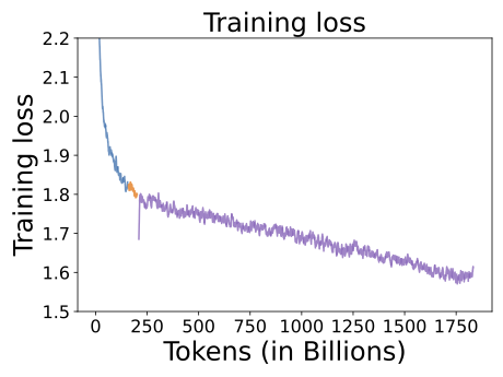
Monitoring the training loss curve gives us the first high-level stability signal. We used TensorBoard to monitor the training loss curve and validation loss curve, as shown in the following figure. The entire model was trained on 1.8 trillion tokens. We observed that the training loss decreases fast for the initial 250 billion tokens and enters a log-linear decrease afterwards.
Monitoring the gradient norm and parameter norms
We monitored the gradient norm as an early signal of divergence. Rapid growth of the gradient norm means (more than three times growth from lowest value) or persistent spikes (benign spikes should return the normal values within a few iterations) can lead to divergence issues. In our training, we observed an ensured gradient norm trending even with BF16, as illustrated in the following figure.

The spikes in our gradient norm often last for a single step and don’t impact the overall training convergence. Specifically, we first tracked a running average (𝑟) of the gradient norm over a window of 20 steps to smooth out the natural fluctuations due to batching. We defined occurrence of a gradient spike when the current gradient norm is higher than 𝑟 + 0.1. Next, we tracked the number of steps for the gradient norm returning to less than 𝑟 + 0.1. Over 86%, the spike deviates from running average for only a single step, as shown in the following figure.

Finally, we also monitored the parameter norm. This metric is a good way to monitor convergence during the initialization stage. For this setup, the initial values are around 1,600, which is expected based on empirical training results from other hardware.

Training results
In this section, we present the results for model quality evaluation and throughput scalability.
Model quality evaluation
The whole training process takes a few weeks. With the saved pre-training model, we benchmarked the model quality based on different tasks and compared it with OpenLlama 2-7B. The following table benchmarks the accuracy over a variety of tasks: MMLU, BBH, common reasoning, world knowledge, reading comprehension, math, and code. For OpenLLaMA 2, we used the available pre-trained weights and evaluated using the same evaluation pipeline as our pre-trained model. Overall, the model trained on Trn1 shows better or comparable accuracy for all tasks except common reasoning.
| Task | Shots | Metric | Llama2-7B on trn1 | OpenLlama-2 |
| MMLU (5 shot) | 5 | accuracy | 41.318 (3.602) | 41.075 (3.611) |
| BBH (3 shot) | 3 | multiple_choice_grade | 36.565 (1.845) | 35.502 (1.861) |
| Common Reasoning | 0 | accuracy | 56.152 (1.194) | 56.893(1.195) |
| . | . | accuracy_norm | 59.455 (1.206) | 61.262(1.19) |
| World Knowledge (5 shot) | Average | exact match | 38.846 (0.534) | 37.023 (0.52) |
| Reading Comprehension | 0 | accuracy | 72.508 (0.781) | 72.416 (0.782) |
| Math | 8 | accuracy | 9.401 (0.804) | 5.231 (0.613) |
| Code | 0 | pass@1 | 7.62 | 9.06 |
| . | . | pass@10 | 19.83 | 23.58 |
| . | . | pass@100 | 34.15 | 40.24 |
We also verified that the model accuracy keeps increasing by training more tokens in the dataset. For comparison, we tracked the model accuracy using saved intermediate checkpoints for different tasks, as shown in the following figures.
The first figure shows the model accuracy for world knowledge.

The following figure shows the model accuracy for common reasoning.

The following figure shows the model accuracy for math.

We observed that the accuracy increases with more training tokens for different tasks.
The model quality could be further improved with fine-tuning for specific tasks based on domain specific dataset.
Throughput scalability
In addition to the model quality, we checked the training throughput scaling and got more than 90% scaling efficiency for Llama 2-70B for 64 instances, as shown in the following figure. The Llama 2-7B scaling efficiency is slightly lower because the model size is relatively small for a cluster at this scale.

Clean up
To clean up all the provisioned resources for this post, use the following code and the cleanup script described in Train Llama2 with AWS Trainium on Amazon EKS:
Conclusion
This post showed the end-to-end training example for the Llama 2-7B model with up to 1.8 tokens of dataset on 128 trn1.32xlarge clusters. We discussed best practices to overcome the challenges associated to this type of large model training: hardware stability and recovery, model training stability and convergence, and throughput optimization. The saved training model demonstrated good model quality for the general tasks and showed great cost benefit training on AI purpose-built Trainium accelerators. To learn more about the model architectures supported for training on Trainium and access tutorials, refer to Training Samples/Tutorials.
Reference
HLAT: High-quality Large Language Model Pre-trained on AWS Trainium, https://arxiv.org/pdf/2404.10630
About the Authors
 Jianying Lang is a Principal Solutions Architect at AWS Worldwide Specialist Organization (WWSO). She has over 15 years of working experience in the HPC and AI field. At AWS, she focuses on helping customers deploy, optimize, and scale their AI/ML workloads on accelerated computing instances. She is passionate about combining the techniques in HPC and AI fields. Jianying holds a PhD in Computational Physics from the University of Colorado at Boulder.
 Fei Chen has 15 years’ industry experiences of leading teams in developing and productizing AI/ML at internet scale. At AWS, she leads the worldwide solution teams in Advanced Compute, including AI accelerators, HPC, IoT, visual and spatial compute, and the emerging technology focusing on technical innovations (AI and generative AI) in the aforementioned domains.
 Haozheng Fan is a software engineer at AWS. He is interested in large language models (LLMs) in production, including pre-training, fine-tuning, and evaluation. His works span from framework application level to hardware kernel level. He currently works on LLM training on novel hardware, with a focus on training efficiency and model quality.
 Hao Zhou is a Research Scientist with Amazon SageMaker. Before that, he worked on developing machine learning methods for fraud detection for Amazon Fraud Detector. He is passionate about applying machine learning, optimization, and generative AI techniques to various real-world problems. He holds a PhD in Electrical Engineering from Northwestern University.
 Yida Wang is a principal scientist in the AWS AI team of Amazon. His research interest is in systems, high-performance computing, and big data analytics. He currently works on deep learning systems, with a focus on compiling and optimizing deep learning models for efficient training and inference, especially large-scale foundation models. The mission is to bridge the high-level models from various frameworks and low-level hardware platforms including CPUs, GPUs, and AI accelerators, so that different models can run in high performance on different devices.
 Jun (Luke) Huan is a Principal Scientist at AWS AI Labs. Dr. Huan works on AI and data science. He has published more than 160 peer-reviewed papers in leading conferences and journals and has graduated 11 PhD students. He was a recipient of the NSF Faculty Early Career Development Award in 2009. Before joining AWS, he worked at Baidu Research as a distinguished scientist and the head of Baidu Big Data Laboratory. He founded StylingAI Inc., an AI startup, and worked as the CEO and Chief Scientist from 2019–2021. Before joining the industry, he was the Charles E. and Mary Jane Spahr Professor in the EECS Department at the University of Kansas. From 2015–2018, he worked as a program director at the US NSF, in charge of its big data program.
- SEO Powered Content & PR Distribution. Get Amplified Today.
- PlatoData.Network Vertical Generative Ai. Empower Yourself. Access Here.
- PlatoAiStream. Web3 Intelligence. Knowledge Amplified. Access Here.
- PlatoESG. Carbon, CleanTech, Energy, Environment, Solar, Waste Management. Access Here.
- PlatoHealth. Biotech and Clinical Trials Intelligence. Access Here.
- Source: https://aws.amazon.com/blogs/machine-learning/end-to-end-llm-training-on-instance-clusters-with-over-100-nodes-using-aws-trainium/
- :has
- :is
- :not
- $UP
- 000
- 1
- 100
- 11
- 12
- 130
- 133
- 15 years
- 15%
- 152
- 16
- 160
- 19
- 195
- 2%
- 20
- 2009
- 206
- 22
- 250
- 345
- 360
- 4
- 455
- 5
- 52
- 7
- 70
- 77
- 8
- 804
- 9
- 98
- a
- About
- accelerate
- accelerated
- accelerators
- access
- accumulation
- accuracy
- Achieve
- achieving
- across
- Activation
- actual
- addition
- Additionally
- address
- adopted
- advanced
- affected
- After
- afterwards
- AI
- AI/ML
- algorithms
- All
- allows
- also
- Amazon
- Amazon EC2
- Amazon Fraud Detector
- Amazon FSx
- Amazon SageMaker
- Amazon Web Services
- among
- an
- analytics
- and
- Another
- Apache
- APIs
- applicable
- Application
- applied
- Applying
- architecture
- architectures
- ARE
- around
- AS
- associated
- At
- attention
- Automatic
- automatically
- available
- average
- award
- AWS
- Bad
- Baidu
- Bandwidth
- based
- batching
- BE
- because
- before
- behavior
- being
- benchmarked
- benchmarks
- benefit
- benefits
- BEST
- best practices
- Better
- between
- Big
- Big Data
- Billion
- Billion tokens
- binary
- Black
- Block
- Blocks
- both
- bottleneck
- bottlenecks
- BRIDGE
- built
- but
- by
- CA
- cache
- CAN
- Capacity
- Career
- catastrophic
- caused
- ceo
- challenges
- challenging
- charge
- Charles
- check
- checked
- checking
- chief
- chose
- clean
- Cluster
- code
- Colorado
- combine
- combining
- Common
- Communication
- comparable
- compared
- comparison
- compatible
- compiled
- compiler
- Completed
- components
- computation
- computational
- Compute
- computing
- conferences
- configurations
- connected
- consists
- constantly
- consumption
- Container
- containing
- contains
- contrast
- Convergence
- converted
- copies
- Core
- Cost
- costly
- Costs
- could
- covered
- CPU
- Current
- Currently
- curve
- custom
- customer
- Customers
- data
- Data Analytics
- data science
- data storage
- datasets
- Days
- decrease
- decreases
- deep
- deep learning
- deep neural networks
- deeper
- Default
- defined
- Degree
- demonstrate
- demonstrated
- Department
- depends
- deploy
- deployed
- described
- details
- Detection
- developing
- Development
- deviation
- Devices
- diagram
- DID
- different
- difficult
- Director
- discuss
- discussed
- Distinguished
- distributed
- distributed training
- Divergence
- Docker
- domain
- domains
- Dont
- download
- downloaded
- dr
- due
- during
- dynamically
- e
- each
- Early
- Effective
- efficiency
- efficient
- efficiently
- electrical engineering
- else
- emerging
- Emerging Technology
- empirically
- enable
- enables
- enabling
- encounter
- end-to-end
- engineer
- Engineering
- enhancement
- enough
- ensured
- Enters
- Entire
- Environment
- especially
- Ether (ETH)
- evaluated
- evaluation
- Even
- example
- Except
- Exercise
- expected
- experience
- Experiences
- experimental
- experiments
- Face
- Failure
- failures
- family
- FAST
- fault
- Features
- few
- field
- Fields
- Figure
- Figures
- File
- Files
- filling
- Finally
- finishing
- First
- Fix
- fluctuations
- Focus
- focuses
- focusing
- followed
- following
- follows
- Footprint
- For
- format
- found
- Foundation
- Founded
- four
- Framework
- frameworks
- fraud
- fraud detection
- frequent
- frequently
- from
- full
- function
- functions
- further
- General
- generated
- generation
- generative
- Generative AI
- get
- getting
- gives
- Global
- Goes
- good
- got
- GPUs
- gradients
- graph
- graphs
- great
- Green
- Growth
- Hardware
- Have
- having
- he
- head
- Health
- helping
- High
- high-level
- high-performance
- high-quality
- higher
- highest
- his
- holds
- host
- HOURS
- How
- How To
- However
- hpc
- HTML
- http
- HTTPS
- Hybrid
- if
- illustrates
- image
- immediate
- Impact
- implementation
- implementations
- import
- important
- improve
- improved
- improving
- in
- Inc.
- included
- includes
- Including
- incorrect
- Increases
- increasing
- industry
- inevitably
- Infrastructure
- initial
- innovations
- inputs
- instance
- instances
- instead
- intensive
- interest
- interested
- Intermediate
- Internet
- interrupted
- intervention
- into
- iot
- issues
- IT
- iterations
- ITS
- jane
- joining
- jpg
- Kansas
- keeps
- Key
- knowledge
- Kubernetes
- laboratory
- Labs
- language
- large
- large-scale
- larger
- Last
- Latency
- latest
- layer
- layers
- lead
- leading
- Leads
- LEARN
- learning
- Led
- Length
- less
- Level
- Library
- linear
- List
- Llama
- llm
- load
- loading
- loads
- local
- Look
- loss
- lower
- lowering
- lowest
- machine
- machine learning
- maintain
- make
- MAKES
- manage
- managed
- management
- manual
- many
- mary
- math
- Matrix
- maximum
- means
- mechanisms
- Memory
- message
- Meta
- method
- methods
- metric
- million
- minimum
- Mission
- mixed
- model
- models
- modified
- Monitor
- monitored
- monitoring
- more
- most
- Most Popular
- much
- multiple
- Natural
- Need
- networking
- networks
- Neural
- neural networks
- next
- node
- nodes
- normal
- Northwestern University
- novel
- NSF
- number
- numbers
- numerical
- observed
- occurrence
- of
- offline
- often
- on
- ONE
- online
- only
- open
- open source
- operation
- Operations
- optimal
- optimization
- optimizations
- Optimize
- optimized
- Optimizes
- optimizing
- or
- organization
- original
- OS
- Other
- our
- out
- output
- over
- overall
- Overcome
- overhead
- package
- packaging
- papers
- Parallel
- parameter
- parameters
- particularly
- passionate
- path
- peer-reviewed
- per
- perform
- performance
- performs
- phd
- Physics
- pipeline
- Platforms
- plato
- Plato Data Intelligence
- PlatoData
- plot
- pods
- Popular
- Post
- practices
- Precision
- present
- preserving
- Principal
- problems
- procedure
- process
- processed
- Production
- Professor
- profiling
- Program
- projections
- proven
- provides
- published
- quality
- ranging
- rapid
- Rate
- Raw
- reached
- Reaches
- Reading
- real world
- reasoning
- recommended
- Recover
- recovering
- recovery
- reduce
- reduces
- reducing
- refer
- registry
- relatively
- replaced
- required
- requires
- research
- Resources
- resulted
- Results
- return
- returning
- root
- rounding
- Run
- running
- runs
- runtime
- sagemaker
- same
- saved
- saving
- Scalability
- Scale
- scaled
- scaling
- Science
- Scientist
- scratch
- script
- scrutiny
- sdk
- seconds
- Section
- select
- selection
- SELF
- send
- separate
- Sequence
- Services
- set
- setting
- settings
- setup
- Share
- shared
- she
- shot
- should
- show
- showed
- shown
- Shows
- Signal
- significantly
- similar
- Simple
- single
- Size
- slightly
- small
- smaller
- smooth
- So
- Software
- Software Engineer
- solution
- Solutions
- some
- Source
- Space
- span
- Spatial
- special
- specialist
- specializes
- specific
- specifically
- spike
- spikes
- square
- Stability
- Stage
- standard
- startup
- States
- Step
- Steps
- Stops
- storage
- stored
- storing
- strategies
- Strategy
- stream
- Students
- such
- Supported
- Supporting
- Supports
- sure
- synchronization
- system
- Systems
- table
- takes
- tasks
- team
- teams
- Technical
- technically
- technique
- techniques
- Technology
- test
- text
- than
- that
- The
- their
- Them
- then
- therefore
- These
- this
- those
- three
- Through
- throughput
- time
- times
- to
- token
- Tokenization
- Tokens
- tools
- totaling
- tp
- tracked
- Train
- trained
- Training
- transformer
- tremendous
- trending
- Trillion
- trillions
- tuned
- tutorials
- two
- type
- understanding
- unique
- university
- uploaded
- uptime
- us
- use
- used
- uses
- using
- utilization
- validation
- value
- Values
- variable
- variants
- variety
- various
- verified
- version
- visual
- volume
- want
- warning
- was
- Way..
- we
- web
- web services
- Weeks
- weight
- WELL
- were
- What
- What is
- when
- whereas
- which
- whole
- will
- window
- with
- within
- without
- worked
- worker
- workers
- working
- works
- world
- worldwide
- writer
- X
- years
- yellow
- yields
- you
- zephyrnet