Coletar e anotar dados de imagem é uma das tarefas que mais consomem recursos em qualquer projeto de visão computacional. Pode levar meses para coletar, analisar e experimentar totalmente os fluxos de imagem no nível necessário para competir no mercado atual. Mesmo depois de coletar dados com sucesso, você ainda terá um fluxo constante de erros de anotação, imagens mal enquadradas, pequenas quantidades de dados significativos em um mar de capturas indesejadas e muito mais. Esses principais gargalos são o motivo pelo qual a criação de dados sintéticos precisa estar no kit de ferramentas de todo engenheiro moderno. Ao criar representações 3D dos objetos que queremos modelar, podemos rapidamente prototipar algoritmos enquanto coletamos dados ao vivo simultaneamente.
Neste post, apresento um exemplo de uso da biblioteca de animação de código aberto Blender para criar um pipeline de dados sintéticos de ponta a ponta, usando nuggets de frango como exemplo. A imagem a seguir é uma ilustração dos dados gerados nesta postagem do blog.
O que é Blender?
liqüidificador é um software gráfico 3D de código aberto usado principalmente em animação, impressão 3D e realidade virtual. Ele possui um conjunto de rigging, animação e simulação extremamente abrangente que permite a criação de mundos 3D para praticamente qualquer caso de uso de visão computacional. Ele também possui uma comunidade de suporte extremamente ativa, onde a maioria, se não todos, os erros do usuário são resolvidos.
Configure seu ambiente local
Instalamos duas versões do Blender: uma em uma máquina local com acesso a uma GUI, e outra em um Amazon Elastic Compute Nuvem (Amazon EC2) instância P2.
Instale o Blender e o ZPY
Instale o Blender a partir do Site do Blender.
Em seguida, conclua as seguintes etapas:
- Execute os seguintes comandos:
wget https://mirrors.ocf.berkeley.edu/blender/release/Blender3.2/blender-3.2.0-linux-x64.tar.xz
sudo tar -Jxf blender-3.2.0-linux-x64.tar.xz --strip-components=1 -C /bin
rm -rf blender*

/bin/3.2/python/bin/python3.10 -m ensurepip
/bin/3.2/python/bin/python3.10 -m pip install --upgrade pip
- Copie os cabeçalhos necessários do Python na versão do Blender do Python para que você possa usar outras bibliotecas que não sejam do Blender:
wget https://www.python.org/ftp/python/3.10.2/Python-3.10.2.tgz
tar -xzf Python-3.10.2.tgz
sudo cp Python-3.10.2/Include/* /bin/3.2/python/include/python3.10
- Substitua sua versão do Blender e force as instalações para que o Python fornecido pelo Blender funcione:
/bin/3.2/python/bin/python3.10 -m pip install pybind11 pythran Cython numpy==1.22.1
sudo /bin/3.2/python/bin/python3.10 -m pip install -U Pillow --force
sudo /bin/3.2/python/bin/python3.10 -m pip install -U scipy --force
sudo /bin/3.2/python/bin/python3.10 -m pip install -U shapely --force
sudo /bin/3.2/python/bin/python3.10 -m pip install -U scikit-image --force
sudo /bin/3.2/python/bin/python3.10 -m pip install -U gin-config --force
sudo /bin/3.2/python/bin/python3.10 -m pip install -U versioneer --force
sudo /bin/3.2/python/bin/python3.10 -m pip install -U shapely --force
sudo /bin/3.2/python/bin/python3.10 -m pip install -U ptvsd --force
sudo /bin/3.2/python/bin/python3.10 -m pip install -U ptvseabornsd --force
sudo /bin/3.2/python/bin/python3.10 -m pip install -U zmq --force
sudo /bin/3.2/python/bin/python3.10 -m pip install -U pyyaml --force
sudo /bin/3.2/python/bin/python3.10 -m pip install -U requests --force
sudo /bin/3.2/python/bin/python3.10 -m pip install -U click --force
sudo /bin/3.2/python/bin/python3.10 -m pip install -U table-logger --force
sudo /bin/3.2/python/bin/python3.10 -m pip install -U tqdm --force
sudo /bin/3.2/python/bin/python3.10 -m pip install -U pydash --force
sudo /bin/3.2/python/bin/python3.10 -m pip install -U matplotlib --force
- Baixar
zpy e instale a partir da fonte:
git clone https://github.com/ZumoLabs/zpy
cd zpy
vi requirements.txt
- Altere a versão do NumPy para
>=1.19.4 e scikit-image>=0.18.1 para fazer a instalação 3.10.2 possível e para que você não sobrescreva:
numpy>=1.19.4
gin-config>=0.3.0
versioneer
scikit-image>=0.18.1
shapely>=1.7.1
ptvsd>=4.3.2
seaborn>=0.11.0
zmq
pyyaml
requests
click
table-logger>=0.3.6
tqdm
pydash
- Para garantir a compatibilidade com o Blender 3.2, acesse
zpy/render.py e comente as duas linhas a seguir (para mais informações, consulte Falha do Blender 3.0 #54):
#scene.render.tile_x = tile_size
#scene.render.tile_y = tile_size
- Em seguida, instale o
zpy biblioteca:
/bin/3.2/python/bin/python3.10 setup.py install --user
/bin/3.2/python/bin/python3.10 -c "import zpy; print(zpy.__version__)"
- Baixe a versão complementar do
zpy do GitHub repo para que você possa executar ativamente sua instância:
cd ~
curl -O -L -C - "https://github.com/ZumoLabs/zpy/releases/download/v1.4.1rc9/zpy_addon-v1.4.1rc9.zip"
sudo unzip zpy_addon-v1.4.1rc9.zip -d /bin/3.2/scripts/addons/
mkdir .config/blender/
mkdir .config/blender/3.2
mkdir .config/blender/3.2/scripts
mkdir .config/blender/3.2/scripts/addons/
mkdir .config/blender/3.2/scripts/addons/zpy_addon/
sudo cp -r zpy/zpy_addon/* .config/blender/3.2/scripts/addons/zpy_addon/
- Salve um arquivo chamado
enable_zpy_addon.py na sua /home diretório e execute o comando de ativação, porque você não tem uma GUI para ativá-lo:
import bpy, os
p = os.path.abspath('zpy_addon-v1.4.1rc9.zip')
bpy.ops.preferences.addon_install(overwrite=True, filepath=p)
bpy.ops.preferences.addon_enable(module='zpy_addon')
bpy.ops.wm.save_userpref()

sudo blender -b -y --python enable_zpy_addon.py
If zpy-addon não instala (por qualquer motivo), você pode instalá-lo através da GUI.
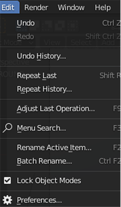
- No Blender, no Editar menu, escolha Preferencias.
- Escolha Add-ons no painel de navegação e ative
zpy.

Você deverá ver uma página aberta na GUI e poderá escolher ZPY. Isso confirmará que o Blender está carregado.

AliceVision e Meshroom
Instale o AliceVision e o Meshroom de seus respectivos repositórios do GitHub:
FFmpeg
Seu sistema deve ter ffmpeg, mas se isso não acontecer, você precisará download .
Malhas instantâneas
Você pode compilar a biblioteca você mesmo ou baixar os binários pré-compilados disponíveis (que foi o que eu fiz) para Malhas instantâneas.
Configure seu ambiente AWS
Agora configuramos o ambiente da AWS em uma instância do EC2. Repetimos os passos da seção anterior, mas apenas para Blender e zpy.
- No console do Amazon EC2, escolha Iniciar instâncias.
- Escolha sua AMI. Existem algumas opções aqui. Podemos escolher uma imagem padrão do Ubuntu, escolher uma instância de GPU e, em seguida, instalar manualmente os drivers e configurar tudo, ou podemos seguir o caminho mais fácil e começar com uma AMI de Deep Learning pré-configurada e nos preocupar apenas em instalar o Blender. post, eu uso a segunda opção e escolho a versão mais recente do Deep Learning AMI para Ubuntu (Versão de Deep Learning AMI (Ubuntu 18.04) 61.0).
- Escolha Tipo de instância¸ escolher p2.xlarg.
- Se você não tiver um par de chaves, crie um novo ou escolha um existente.
- Para esta postagem, use as configurações padrão para rede e armazenamento.
- Escolha Iniciar instâncias.
- Escolha Contato e encontre as instruções para fazer login em nossa instância do SSH no Cliente SSH aba.
- Conecte-se com SSH:
ssh -i "your-pem" ubuntu@IPADDRESS.YOUR-REGION.compute.amazonaws.com
Depois de se conectar à sua instância, siga as mesmas etapas de instalação da seção anterior para instalar o Blender e zpy.
Coleta de dados: digitalização 3D de nossa pepita
Para esta etapa, uso um iPhone para gravar um vídeo de 360 graus em um ritmo bastante lento em torno da minha pepita. Enfiei um nugget de frango em um palito e prendi o palito na minha bancada, e simplesmente girei minha câmera ao redor do nugget para obter o máximo de ângulos que conseguisse. Quanto mais rápido você filmar, menor a probabilidade de obter boas imagens para trabalhar, dependendo da velocidade do obturador.
Depois que terminei de filmar, enviei o vídeo para o meu e-mail e extraí o vídeo para uma unidade local. A partir daí, usei ffmepg para cortar o vídeo em quadros para facilitar muito a ingestão do Meshroom:
mkdir nugget_images
ffmpeg -i VIDEO.mov ffmpeg nugget_images/nugget_%06d.jpg
Abra o Meshroom e use a GUI para arrastar o nugget_images pasta para o painel à esquerda. A partir daí, escolha Início e espere algumas horas (ou menos) dependendo da duração do vídeo e se você tiver uma máquina habilitada para CUDA.

Você deve ver algo como a captura de tela a seguir quando estiver quase completo.

Coleta de dados: manipulação do Blender
Quando a reconstrução do Meshroom estiver concluída, conclua as etapas a seguir:
- Abra a GUI do Blender e no Envie o menu, escolha importação, Em seguida, escolha Frente de onda (obj) para o arquivo de textura criado do Meshroom.
O arquivo deve ser salvo em path/to/MeshroomCache/Texturing/uuid-string/texturedMesh.obj.
- Carregue o arquivo e observe a monstruosidade que é seu objeto 3D.

Aqui é onde fica um pouco complicado.
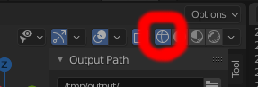
- Role até o canto superior direito e escolha o wireframe ícone em Sombreamento da janela de visualização.
- Selecione seu objeto na viewport direita e certifique-se de que esteja realçado, role até a viewport de layout principal e pressione Aba ou escolha manualmente Modo de edição.

- Em seguida, manobre a janela de visualização de forma a permitir que você veja seu objeto com o mínimo possível atrás dele. Você terá que fazer isso algumas vezes para realmente acertar.
- Clique e arraste uma caixa delimitadora sobre o objeto para que apenas a pepita seja realçada.
- Depois de destacado como na captura de tela a seguir, separamos nossa pepita da massa 3D clicando com o botão esquerdo, escolhendo Separado, e depois Seleção.

Agora vamos para a direita, onde devemos ver dois objetos texturizados: texturedMesh e texturedMesh.001.
- Nosso novo objeto deve ser
texturedMesh.001, então escolhemos texturedMesh e escolha Apagar para remover a massa indesejada.

- Escolha o objeto (
texturedMesh.001) à direita, vá para o nosso visualizador e escolha o objeto, Definir origem e Origem ao centro de massa.

Agora, se quisermos, podemos mover nosso objeto para o centro da viewport (ou simplesmente deixá-lo onde está) e visualizá-lo em toda a sua glória. Observe o grande buraco negro de onde não conseguimos uma boa cobertura de filme! Vamos precisar corrigir isso.

Para limpar nosso objeto de qualquer impureza de pixel, exportamos nosso objeto para um arquivo .obj. Certifique-se de escolher Apenas seleção ao exportar.

Coleta de dados: limpe com malhas instantâneas
Agora temos dois problemas: nossa imagem tem uma lacuna de pixel criada por nossa má filmagem que precisamos limpar, e nossa imagem é incrivelmente densa (o que tornará a geração de imagens extremamente demorada). Para resolver os dois problemas, precisamos usar um software chamado Instant Meshes para extrapolar nossa superfície de pixel para cobrir o buraco negro e também reduzir o objeto total para um tamanho menor e menos denso.
- Abra as malhas instantâneas e carregue nossos arquivos salvos recentemente
nugget.obj arquivo.

- Debaixo Campo de orientação, escolha Resolver.

- Debaixo Campo de posição, escolha Resolver.
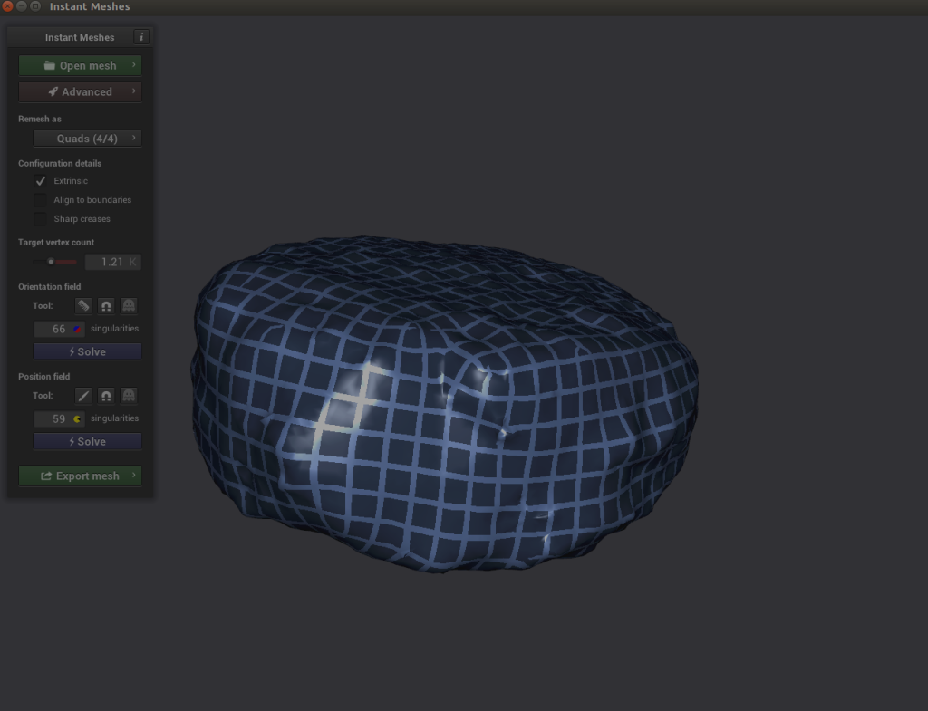 Aqui é onde fica interessante. Se você explorar seu objeto e perceber que as linhas cruzadas do Solucionador de posição parecem desconexas, você pode escolher o ícone de pente em Campo de orientação e redesenhe as linhas corretamente.
- Escolha Resolver tanto Campo de orientação e Campo de posição.

- Se tudo estiver bem, exporte a malha, nomeie-a como
nugget_refined.obj, e salve-o em disco.
Coleta de dados: Agite e asse!
Como nossa malha low-poly não tem nenhuma textura de imagem associada a ela e nossa malha high-poly tem, precisamos assar a textura high-poly na malha low-poly ou criar uma nova textura e atribuí-la a nosso objeto. Para simplificar, vamos criar uma textura de imagem do zero e aplicá-la ao nosso nugget.
Usei a pesquisa de imagens do Google para pepitas e outras coisas fritas para obter uma imagem de alta resolução da superfície de um objeto frito. Encontrei uma imagem super em alta resolução de um queijo coalho frito e fiz uma nova imagem cheia de textura frita.

Com esta imagem, estou pronto para concluir as seguintes etapas:
- Abra o Blender e carregue o novo
nugget_refined.obj da mesma forma que você carregou seu objeto inicial: no Envie o menu, escolha importação, Frente de onda (obj)e escolha o nugget_refined.obj arquivo.
- Em seguida, vá para o Sombreamento aba.
Na parte inferior você deve observar duas caixas com os títulos Princípio BDSF e Saída de Materiais.
- No Adicionar menu, escolha Textura e Textura da imagem.
An Textura da imagem caixa deve aparecer.
- Escolha Abrir imagem e carregue sua imagem de textura frita.
- Arraste o mouse entre Cor no Textura da imagem caixa e Cor base no Princípio BDSF caixa.

Agora sua pepita deve estar pronta!
Coleta de dados: crie variáveis de ambiente do Blender
Agora que temos nosso objeto nugget base, precisamos criar algumas coleções e variáveis de ambiente para nos ajudar em nosso processo.
- Clique com o botão esquerdo na área da cena da mão e escolha Nova coleção.
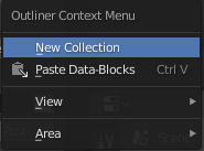
- Crie as seguintes coleções: ORIGEM, PEPITA e GERADO.

- Arraste a pepita para o PEPITA coleção e renomeie-a pepita_base.
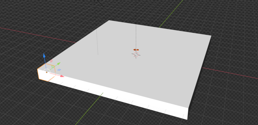
Coleta de dados: criar um avião
Vamos criar um objeto de fundo a partir do qual nossos nuggets serão gerados quando estivermos renderizando imagens. Em um caso de uso do mundo real, esse plano é onde nossas pepitas são colocadas, como uma bandeja ou caixa.
- No Adicionar menu, escolha Malha e depois Avião.
A partir daqui, vamos para o lado direito da página e encontramos a caixa laranja (Propriedades do objeto).
- No Transformar painel, para XYZ Eulerconjunto X para 46.968, Y para 46.968, e Z para 1.0.
- Para ambos Localização e rotaçãoconjunto X, Y e Z para 0.

Coleta de dados: Defina a câmera e o eixo
Em seguida, vamos configurar nossas câmeras corretamente para que possamos gerar imagens.
- No Adicionar menu, escolha vazio e Eixo Simples.
- Nomeie o objeto Eixo Principal.

- Certifique-se de que nosso eixo seja 0 para todas as variáveis (para que fique diretamente no centro).

- Se você já tiver uma câmera criada, arraste-a para o eixo principal.
- Escolha item e Transformar.
- Escolha Localizaçãoconjunto X para 0, Y para 0, e Z para 100.

Coleta de dados: Lá vem o sol
Em seguida, adicionamos um objeto Sun.
- No Adicionar menu, escolha Claro e Espreguiçadeiras.
A localização deste objeto não importa necessariamente, desde que esteja centralizado em algum lugar sobre o objeto plano que definimos.
- Escolha o ícone de lâmpada verde no painel inferior direito (Propriedades de dados do objeto) e defina a intensidade para 5.0.
- Repita o mesmo procedimento para adicionar um Claro objeto e colocá-lo em um ponto aleatório sobre o plano.

Coleta de dados: baixe fundos aleatórios
Para injetar aleatoriedade em nossas imagens, baixamos tantas texturas aleatórias de textura.ninja como podemos (por exemplo, tijolos). Faça o download para uma pasta em seu espaço de trabalho chamada random_textures. Baixei cerca de 50.

Gerar imagens
Agora vamos ao que interessa: gerar imagens.
Pipeline de geração de imagens: Object3D e DensityController
Vamos começar com algumas definições de código:
class Object3D:
	'''
	object container to store mesh information about the
	given object

	Returns
	the Object3D object
	'''
	def __init__(self, object: Union[bpy.types.Object, str]):
		"""Creates a Object3D object.

		Args:
		obj (Union[bpy.types.Object, str]): Scene object (or it's name)
		"""
		self.object = object
		self.obj_poly = None
		self.mat = None
		self.vert = None
		self.poly = None
		self.bvht = None
		self.calc_mat()
		self.calc_world_vert()
		self.calc_poly()
		self.calc_bvht()

	def calc_mat(self) -> None:
		"""store an instance of the object's matrix_world"""
		self.mat = self.object.matrix_world

	def calc_world_vert(self) -> None:
		"""calculate the verticies from object's matrix_world perspective"""
		self.vert = [self.mat @ v.co for v in self.object.data.vertices]
		self.obj_poly = np.array(self.vert)

	def calc_poly(self) -> None:
		"""store an instance of the object's polygons"""
		self.poly = [p.vertices for p in self.object.data.polygons]

	def calc_bvht(self) -> None:
		"""create a BVHTree from the object's polygon"""
		self.bvht = BVHTree.FromPolygons( self.vert, self.poly )

	def regenerate(self) -> None:
		"""reinstantiate the object's variables;
		used when the object is manipulated after it's creation"""
		self.calc_mat()
		self.calc_world_vert()
		self.calc_poly()
		self.calc_bvht()

	def __repr__(self):
		return "Object3D: " + self.object.__repr__()
Primeiro definimos uma classe de contêiner básica com algumas propriedades importantes. Esta classe existe principalmente para nos permitir criar uma árvore BVH (uma forma de representar nosso objeto pepita no espaço 3D), onde precisaremos usar o BVHTree.overlap método para ver se dois objetos pepita gerados independentes estão sobrepostos em nosso espaço 3D. Mais sobre isso mais tarde.
A segunda parte do código é o nosso controlador de densidade. Isso serve como uma maneira de nos vincularmos às regras da realidade e não ao mundo 3D. Por exemplo, no mundo do Blender 3D, os objetos no Blender podem existir uns dentro dos outros; no entanto, a menos que alguém esteja realizando alguma ciência estranha em nossos nuggets de frango, queremos garantir que não haja dois nuggets sobrepostos em um grau que o torne visualmente irreal.
Nós usamos nosso Plane objeto para gerar um conjunto de cubos invisíveis limitados que podem ser consultados a qualquer momento para ver se o espaço está ocupado ou não.

Veja o seguinte código:
class DensityController:
    """Container that controlls the spacial relationship between 3D objects

    Returns:
        DensityController: The DensityController object.
    """
    def __init__(self):
        self.bvhtrees = None
        self.overlaps = None
        self.occupied = None
        self.unoccupied = None
        self.objects3d = []

    def auto_generate_kdtree_cubes(
        self,
        num_objects: int = 100, # max size of nuggets
    ) -> None:
        """
        function to generate physical kdtree cubes given a plane of -resize- size
        this allows us to access each cube's overlap/occupancy status at any given
        time

        creates a KDTree collection, a cube, a set of individual cubes, and the
        BVHTree object for each individual cube

        Args:
            resize (Tuple[float]): the size of a cube to create XYZ.
            cuts (int): how many cuts are made to the cube face
                12 cuts == 13 Rows x 13 Columns
        """
No snippet a seguir, selecionamos o nugget e criamos um cubo delimitador em torno desse nugget. Este cubo representa o tamanho de um único pseudo-voxel do nosso objeto psuedo-kdtree. Precisamos usar o bpy.context.view_layer.update() função porque quando este código está sendo executado de dentro de uma função ou script versus o blender-gui, parece que o view_layer não é atualizado automaticamente.
        # read the nugget,
        # see how large the cube needs to be to encompass a single nugget
        # then touch a parameter to allow it to be smaller or larger (eg more touching)
        bpy.context.view_layer.objects.active = bpy.context.scene.objects.get('nugget_base')
        bpy.ops.object.origin_set(type='ORIGIN_GEOMETRY', center='BOUNDS')
        #create a cube for the bounding box
        bpy.ops.mesh.primitive_cube_add(location=Vector((0,0,0)))
        #our new cube is now the active object, so we can keep track of it in a variable:
        bound_box = bpy.context.active_object
        bound_box.name = 'CUBE1'
        bpy.context.view_layer.update()
        #copy transforms
        nug_dims = bpy.data.objects["nugget_base"].dimensions
        bpy.data.objects["CUBE1"].dimensions = nug_dims
        bpy.context.view_layer.update()
        bpy.data.objects["CUBE1"].location = bpy.data.objects["nugget_base"].location
        bpy.context.view_layer.update()
        bpy.data.objects["CUBE1"].rotation_euler = bpy.data.objects["nugget_base"].rotation_euler
        bpy.context.view_layer.update()
        print("bound_box.dimensions: ", bound_box.dimensions)
        print("bound_box.location:", bound_box.location)
Em seguida, atualizamos ligeiramente nosso objeto cubo para que seu comprimento e largura sejam quadrados, em oposição ao tamanho natural do nugget do qual foi criado:
        # this cube created isn't always square, but we're going to make it square
        # to fit into our
        x, y, z = bound_box.dimensions
        v = max(x, y)
        if np.round(v) < v:
            v = np.round(v)+1
        bb_x, bb_y = v, v
        bound_box.dimensions = Vector((v, v, z))
        bpy.context.view_layer.update()
        print("bound_box.dimensions updated: ", bound_box.dimensions)
        # now we generate a plane
        # calc the size of the plane given a max number of boxes.
Agora usamos nosso objeto de cubo atualizado para criar um plano que pode conter volumetricamente num_objects quantidade de pepitas:
        x, y, z = bound_box.dimensions
        bb_loc = bound_box.location
        bb_rot_eu = bound_box.rotation_euler
        min_area = (x*y)*num_objects
        min_length = min_area / num_objects
        print(min_length)
        # now we generate a plane
        # calc the size of the plane given a max number of boxes.
        bpy.ops.mesh.primitive_plane_add(location=Vector((0,0,0)), size = min_length)
        plane = bpy.context.selected_objects[0]
        plane.name = 'PLANE'
        # move our plane to our background collection
        # current_collection = plane.users_collection
        link_object('PLANE', 'BACKGROUND')
        bpy.context.view_layer.update()
Pegamos nosso objeto plano e criamos um cubo gigante do mesmo comprimento e largura do nosso plano, com a altura do nosso cubo pepita, CUBO1:
        # New Collection
        my_coll = bpy.data.collections.new("KDTREE")
        # Add collection to scene collection
        bpy.context.scene.collection.children.link(my_coll)
        # now we generate cubes based on the size of the plane.
        bpy.ops.mesh.primitive_cube_add(location=Vector((0,0,0)), size = min_length)
        bpy.context.view_layer.update()
        cube = bpy.context.selected_objects[0]
        cube_dimensions = cube.dimensions
        bpy.context.view_layer.update()
        cube.dimensions = Vector((cube_dimensions[0], cube_dimensions[1], z))
        bpy.context.view_layer.update()
        cube.location = bb_loc
        bpy.context.view_layer.update()
        cube.rotation_euler = bb_rot_eu
        bpy.context.view_layer.update()
        cube.name = 'cube'
        bpy.context.view_layer.update()
        current_collection = cube.users_collection
        link_object('cube', 'KDTREE')
        bpy.context.view_layer.update()
A partir daqui, queremos criar voxels do nosso cubo. Tomamos o número de cubos que caberiam num_objects e, em seguida, corte-os do nosso objeto cubo. Procuramos a face de malha voltada para cima do nosso cubo e, em seguida, escolhemos essa face para fazer nossos cortes. Veja o seguinte código:
        # get the bb volume and make the proper cuts to the object
        bb_vol = x*y*z
        cube_vol = cube_dimensions[0]*cube_dimensions[1]*cube_dimensions[2]
        n_cubes = cube_vol / bb_vol
        cuts = n_cubes / ((x+y) / 2)
        cuts = int(np.round(cuts)) - 1 #
        # select the cube
        for object in bpy.data.objects:
            object.select_set(False)
        bpy.context.view_layer.update()
        for object in bpy.data.objects:
            object.select_set(False)
        bpy.data.objects['cube'].select_set(True) # Blender 2.8x
        bpy.context.view_layer.objects.active = bpy.context.scene.objects.get('cube')
        # set to edit mode
        bpy.ops.object.mode_set(mode='EDIT', toggle=False)
        print('edit mode success')
        # get face_data
        context = bpy.context
        obj = context.edit_object
        me = obj.data
        mat = obj.matrix_world
        bm = bmesh.from_edit_mesh(me)
        up_face = None
        # select upwards facing cube-face
        # https://blender.stackexchange.com/questions/43067/get-a-face-selected-pointing-upwards
        for face in bm.faces:
            if (face.normal-UP_VECTOR).length < EPSILON:
                up_face = face
                break
        assert(up_face)
        # subdivide the edges to get the perfect kdtree cubes
        bmesh.ops.subdivide_edges(bm,
                edges=up_face.edges,
                use_grid_fill=True,
                cuts=cuts)
        bpy.context.view_layer.update()
        # get the center point of each face
Por fim, calculamos o centro da face superior de cada corte que fizemos do nosso cubo grande e criamos cubos reais a partir desses cortes. Cada um desses cubos recém-criados representa um único pedaço de espaço para gerar ou mover pepitas pelo nosso avião. Veja o seguinte código:
        face_data = {}
        sizes = []
        for f, face in enumerate(bm.faces):
            face_data[f] = {}
            face_data[f]['calc_center_bounds'] = face.calc_center_bounds()
            loc = mat @ face_data[f]['calc_center_bounds']
            face_data[f]['loc'] = loc
            sizes.append(loc[-1])
        # get the most common cube-z; we use this to determine the correct loc
        counter = Counter()
        counter.update(sizes)
        most_common = counter.most_common()[0][0]
        cube_loc = mat @ cube.location
        # get out of edit mode
        bpy.ops.object.mode_set(mode='OBJECT', toggle=False)
        # go to new colection
        bvhtrees = {}
        for f in face_data:
            loc = face_data[f]['loc']
            loc = mat @ face_data[f]['calc_center_bounds']
            print(loc)
            if loc[-1] == most_common:
                # set it back down to the floor because the face is elevated to the
                # top surface of the cube
                loc[-1] = cube_loc[-1]
                bpy.ops.mesh.primitive_cube_add(location=loc, size = x)
                cube = bpy.context.selected_objects[0]
                cube.dimensions = Vector((x, y, z))
                # bpy.context.view_layer.update()
                cube.name = "cube_{}".format(f)
                #my_coll.objects.link(cube)
                link_object("cube_{}".format(f), 'KDTREE')
                #bpy.context.view_layer.update()
                bvhtrees[f] = {
                    'occupied' : 0,
                    'object' : Object3D(cube)
                }
        for object in bpy.data.objects:
            object.select_set(False)
        bpy.data.objects['CUBE1'].select_set(True) # Blender 2.8x
        bpy.ops.object.delete()
        return bvhtrees
Em seguida, desenvolvemos um algoritmo que entende quais cubos estão ocupados em um determinado momento, descobre quais objetos se sobrepõem e move objetos sobrepostos separadamente para o espaço desocupado. Não conseguiremos nos livrar de todas as sobreposições inteiramente, mas podemos fazer com que pareça real o suficiente.


Veja o seguinte código:
    def find_occupied_space(
        self,
        objects3d: List[Object3D],
    ) -> None:
        """
        discover which cube's bvhtree is occupied in our kdtree space

        Args:
            list of Object3D objects

        """
        count = 0
        occupied = []
        for i in self.bvhtrees:
            bvhtree = self.bvhtrees[i]['object']
            for object3d in objects3d:
                if object3d.bvht.overlap(bvhtree.bvht):
                    self.bvhtrees[i]['occupied'] = 1

    def find_overlapping_objects(
        self,
        objects3d: List[Object3D],
    ) -> List[Tuple[int]]:
        """
        returns which Object3D objects are overlapping

        Args:
            list of Object3D objects

        Returns:
            List of indicies from objects3d that are overlap
        """
        count = 0
        overlaps = []
        for i, x_object3d in enumerate(objects3d):
            for ii, y_object3d in enumerate(objects3d[i+1:]):
                if x_object3d.bvht.overlap(y_object3d.bvht):
                    overlaps.append((i, ii))
        return overlaps

    def calc_most_overlapped(
        self,
        overlaps: List[Tuple[int]]
    ) -> List[Tuple[int]]:
        """
        Algorithm to count the number of edges each index has
        and return a sorted list from most->least with the number
        of edges each index has.

        Args:
            list of indicies that are overlapping

        Returns:
            list of indicies with the total number of overlapps they have
            [index, count]
        """
        keys = {}
        for x,y in overlaps:
            if x not in keys:
                keys[x] = 0
            if y not in keys:
                keys[y] = 0
            keys[x]+=1
            keys[y]+=1
        # sort by most edges first
        index_counts = sorted(keys.items(), key=lambda x: x[1])[::-1]
        return index_counts

    def get_random_unoccupied(
        self
    ) -> Union[int,None]:
        """
        returns a randomly chosen unoccuped kdtree cube

        Return
            either the kdtree cube's key or None (meaning all spaces are
            currently occupied)
            Union[int,None]
        """
        unoccupied = []
        for i in self.bvhtrees:
            if not self.bvhtrees[i]['occupied']:
                unoccupied.append(i)
        if unoccupied:
            random.shuffle(unoccupied)
            return unoccupied[0]
        else:
            return None

    def regenerate(
        self,
        iterable: Union[None, List[Object3D]] = None
    ) -> None:
        """
        this function recalculates each objects world-view information
        we default to None, which means we're recalculating the self.bvhtree cubes

        Args:
            iterable (None or List of Object3D objects). if None, we default to
            recalculating the kdtree
        """
        if isinstance(iterable, list):
            for object in iterable:
                object.regenerate()
        else:
            for idx in self.bvhtrees:
                self.bvhtrees[idx]['object'].regenerate()
                self.update_tree(idx, occupied=0)

    def process_trees_and_objects(
        self,
        objects3d: List[Object3D],
    ) -> List[Tuple[int]]:
        """
        This function finds all overlapping objects within objects3d,
        calculates the objects with the most overlaps, searches within
        the kdtree cube space to see which cubes are occupied. It then returns
        the edge-counts from the most overlapping objects

        Args:
            list of Object3D objects
        Returns
            this returns the output of most_overlapped
        """
        overlaps = self.find_overlapping_objects(objects3d)
        most_overlapped = self.calc_most_overlapped(overlaps)
        self.find_occupied_space(objects3d)
        return most_overlapped

    def move_objects(
        self,
        objects3d: List[Object3D],
        most_overlapped: List[Tuple[int]],
        z_increase_offset: float = 2.,
    ) -> None:
        """
        This function iterates through most-overlapped, and uses
        the index to extract the matching object from object3d - it then
        finds a random unoccupied kdtree cube and moves the given overlapping
        object to that space. It does this for each index from the most-overlapped
        function

        Args:
            objects3d: list of Object3D objects
            most_overlapped: a list of tuples (index, count) - where index relates to
                where it's found in objects3d and count - how many times it overlaps
                with other objects
            z_increase_offset: this value increases the Z value of the object in order to
                make it appear as though it's off the floor. If you don't augment this value
                the object looks like it's 'inside' the ground plane
        """
        for idx, cnt in most_overlapped:
            object3d = objects3d[idx]
            unoccupied_idx = self.get_random_unoccupied()
            if unoccupied_idx:
                object3d.object.location =  self.bvhtrees[unoccupied_idx]['object'].object.location
                # ensure the nuggest is above the groundplane
                object3d.object.location[-1] = z_increase_offset
                self.update_tree(unoccupied_idx, occupied=1)

    def dynamic_movement(
        self,
        objects3d: List[Object3D],
        tries: int = 100,
        z_offset: float = 2.,
    ) -> None:
        """
        This function resets all objects to get their current positioning
        and randomly moves objects around in an attempt to avoid any object
        overlaps (we don't want two objects to be spawned in the same position)

        Args:
            objects3d: list of Object3D objects
            tries: int the number of times we want to move objects to random spaces
                to ensure no overlaps are present.
            z_offset: this value increases the Z value of the object in order to
                make it appear as though it's off the floor. If you don't augment this value
                the object looks like it's 'inside' the ground plane (see `move_objects`)
        """

        # reset all objects
        self.regenerate(objects3d)
        # regenerate bvhtrees
        self.regenerate(None)

        most_overlapped = self.process_trees_and_objects(objects3d)
        attempts = 0
        while most_overlapped:
            if attempts>=tries:
                break
            self.move_objects(objects3d, most_overlapped, z_offset)
            attempts+=1
            # recalc objects
            self.regenerate(objects3d)
            # regenerate bvhtrees
            self.regenerate(None)
            # recalculate overlaps
            most_overlapped = self.process_trees_and_objects(objects3d)

    def generate_spawn_point(
        self,
    ) -> Vector:
        """
        this function generates a random spawn point by finding which
        of the kdtree-cubes are unoccupied, and returns one of those

        Returns
            the Vector location of the kdtree-cube that's unoccupied
        """
        idx = self.get_random_unoccupied()
        print(idx)
        self.update_tree(idx, occupied=1)
        return self.bvhtrees[idx]['object'].object.location

    def update_tree(
        self,
        idx: int,
        occupied: int,
    ) -> None:
        """
        this function updates the given state (occupied vs. unoccupied) of the
        kdtree given the idx

        Args:
            idx: int
            occupied: int
        """
        self.bvhtrees[idx]['occupied'] = occupied
Pipeline de geração de imagens: corridas legais
Nesta seção, detalhamos o que nossos run função está fazendo.
Inicializamos nosso DensityController e crie algo chamado saver usando o ImageSaver da zpy. Isso nos permite salvar facilmente nossas imagens renderizadas em qualquer local de nossa escolha. Em seguida, adicionamos nosso nugget categoria (e se tivéssemos mais categorias, nós as adicionaríamos aqui). Veja o seguinte código:
@gin.configurable("run")
@zpy.blender.save_and_revert
def run(
    max_num_nuggets: int = 100,
    jitter_mesh: bool = True,
    jitter_nugget_scale: bool = True,
    jitter_material: bool = True,
    jitter_nugget_material: bool = False,
    number_of_random_materials: int = 50,
    nugget_texture_path: str = os.getcwd()+"/nugget_textures",
    annotations_path = os.getcwd()+'/nugget_data',
):
    """
    Main run function.
    """
    density_controller = DensityController()
    # Random seed results in unique behavior
    zpy.blender.set_seed(random.randint(0,1000000000))

    # Create the saver object
    saver = zpy.saver_image.ImageSaver(
        description="Image of the randomized Amazon nuggets",
        output_dir=annotations_path,
    )
    saver.add_category(name="nugget")
Em seguida, precisamos criar um objeto de origem a partir do qual geramos os nuggets de cópia; neste caso, é o nugget_base que criamos:
    # Make a list of source nugget objects
    source_nugget_objects = []
    for obj in zpy.objects.for_obj_in_collections(
        [
            bpy.data.collections["NUGGET"],
        ]
    ):
        assert(obj!=None)

        # pass on everything not named nugget
        if 'nugget_base' not in obj.name:
            print('passing on {}'.format(obj.name))
            continue
        zpy.objects.segment(obj, name="nugget", as_category=True) #color=nugget_seg_color
        print("zpy.objects.segment: check {}".format(obj.name))
        source_nugget_objects.append(obj.name)
Agora que temos nosso nugget base, vamos salvar as poses do mundo (locais) de todos os outros objetos para que, após cada execução de renderização, possamos usar essas poses salvas para reinicializar uma renderização. Também movemos nosso nugget base completamente para fora do caminho para que o kdtree não perceba que um espaço está sendo ocupado. Finalmente, inicializamos nossos objetos kdtree-cube. Veja o seguinte código:
    # move nugget point up 10 z's so it won't collide with base-cube
    bpy.data.objects["nugget_base"].location[-1] = 10

    # Save the position of the camera and light
    # create light and camera
    zpy.objects.save_pose("Camera")
    zpy.objects.save_pose("Sun")
    zpy.objects.save_pose("Plane")
    zpy.objects.save_pose("Main Axis")
    axis = bpy.data.objects['Main Axis']
    print('saving poses')
    # add some parameters to this

    # get the plane-3d object
    plane3d = Object3D(bpy.data.objects['Plane'])

    # generate kdtree cubes
    density_controller.generate_kdtree_cubes()
O código a seguir coleta nossos planos de fundo baixados do texture.ninja, onde eles serão usados para serem projetados aleatoriamente em nosso avião:
    # Pre-create a bunch of random textures
    #random_materials = [
    #    zpy.material.random_texture_mat() for _ in range(number_of_random_materials)
    #]
    p = os.path.abspath(os.getcwd()+'/random_textures')
    print(p)
    random_materials = []
    for x in os.listdir(p):
        texture_path = Path(os.path.join(p,x))
        y = zpy.material.make_mat_from_texture(texture_path, name=texture_path.stem)
        random_materials.append(y)
    #print(random_materials[0])

    # Pre-create a bunch of random textures
    random_nugget_materials = [
        random_nugget_texture_mat(Path(nugget_texture_path)) for _ in range(number_of_random_materials)
    ]
Aqui é onde a magia começa. Primeiro, regeneramos kdtree-cubes para esta execução para que possamos começar de novo:
    # Run the sim.
    for step_idx in zpy.blender.step():
        density_controller.generate_kdtree_cubes()

        objects3d = []
        num_nuggets = random.randint(40, max_num_nuggets)
        log.info(f"Spawning {num_nuggets} nuggets.")
        spawned_nugget_objects = []
        for _ in range(num_nuggets):
Usamos nosso controlador de densidade para gerar um ponto de spawn aleatório para nosso nugget, criamos uma cópia de nugget_base, e mova a cópia para o ponto de spawn gerado aleatoriamente:
            # Choose location to spawn nuggets
            spawn_point = density_controller.generate_spawn_point()
            # manually spawn above the floor
            # spawn_point[-1] = 1.8 #2.0

            # Pick a random object to spawn
            _name = random.choice(source_nugget_objects)
            log.info(f"Spawning a copy of source nugget {_name} at {spawn_point}")
            obj = zpy.objects.copy(
                bpy.data.objects[_name],
                collection=bpy.data.collections["SPAWNED"],
                is_copy=True,
            )

            obj.location = spawn_point
            obj.matrix_world = mathutils.Matrix.Translation(spawn_point)
            spawned_nugget_objects.append(obj)
Em seguida, agitamos aleatoriamente o tamanho da pepita, a malha da pepita e a escala da pepita para que não haja duas pepitas iguais:
            # Segment the newly spawned nugget as an instance
            zpy.objects.segment(obj)

            # Jitter final pose of the nugget a little
            zpy.objects.jitter(
                obj,
                rotate_range=(
                    (0.0, 0.0),
                    (0.0, 0.0),
                    (-math.pi * 2, math.pi * 2),
                ),
            )

            if jitter_nugget_scale:
                # Jitter the scale of each nugget
                zpy.objects.jitter(
                    obj,
                    scale_range=(
                        (0.8, 2.0), #1.2
                        (0.8, 2.0), #1.2
                        (0.8, 2.0), #1.2
                    ),
                )

            if jitter_mesh:
                # Jitter (deform) the mesh of each nugget
                zpy.objects.jitter_mesh(
                    obj=obj,
                    scale=(
                        random.uniform(0.01, 0.03),
                        random.uniform(0.01, 0.03),
                        random.uniform(0.01, 0.03),
                    ),
                )

            if jitter_nugget_material:
                # Jitter the material (apperance) of each nugget
                for i in range(len(obj.material_slots)):
                    obj.material_slots[i].material = random.choice(random_nugget_materials)
                    zpy.material.jitter(obj.material_slots[i].material)
Transformamos nossa cópia de pepita em um Object3D objeto onde usamos a funcionalidade de árvore BVH para ver se nosso plano cruza ou se sobrepõe a qualquer face ou vértice em nossa cópia do nugget. Se encontrarmos uma sobreposição com o plano, simplesmente movemos a pepita para cima em seu eixo Z. Veja o seguinte código:
            # create 3d obj for movement
            nugget3d = Object3D(obj)

            # make sure the bottom most part of the nugget is NOT
            # inside the plane-object
            plane_overlap(plane3d, nugget3d)

            objects3d.append(nugget3d)
Agora que todos os nuggets foram criados, usamos nosso DensityController para mover as pepitas para que tenhamos um número mínimo de sobreposições, e aquelas que se sobrepõem não são horríveis:
        # ensure objects aren't on top of each other
        density_controller.dynamic_movement(objects3d)
No código a seguir: restauramos o Camera e Main Axis poses e selecione aleatoriamente a que distância a câmera está Plane objeto:
        # Return camera to original position
        zpy.objects.restore_pose("Camera")
        zpy.objects.restore_pose("Main Axis")
        zpy.objects.restore_pose("Camera")
        zpy.objects.restore_pose("Main Axis")

        # assert these are the correct versions...
        assert(bpy.data.objects["Camera"].location == Vector((0,0,100)))
        assert(bpy.data.objects["Main Axis"].location == Vector((0,0,0)))
        assert(bpy.data.objects["Main Axis"].rotation_euler == Euler((0,0,0)))

        # alter the Z ditance with the camera
        bpy.data.objects["Camera"].location = (0, 0, random.uniform(0.75, 3.5)*100)
Nós decidimos quão aleatoriamente queremos que a câmera viaje ao longo do Main Axis. Dependendo se queremos que ele fique principalmente acima da cabeça ou se nos importamos muito com o ângulo de visão do tabuleiro, podemos ajustar o top_down_mostly parâmetro dependendo de quão bem nosso modelo de treinamento está captando o sinal de “O que é mesmo uma pepita de qualquer maneira?”
        # alter the main-axis beta/gamma params
        top_down_mostly = False
        if top_down_mostly:
            zpy.objects.rotate(
                bpy.data.objects["Main Axis"],
                rotation=(
                    random.uniform(0.05, 0.05),
                    random.uniform(0.05, 0.05),
                    random.uniform(0.05, 0.05),
                ),
            )
        else:
            zpy.objects.rotate(
                bpy.data.objects["Main Axis"],
                rotation=(
                    random.uniform(-1., 1.),
                    random.uniform(-1., 1.),
                    random.uniform(-1., 1.),
                ),
            )

        print(bpy.data.objects["Main Axis"].rotation_euler)
        print(bpy.data.objects["Camera"].location)
No código a seguir, fazemos a mesma coisa com o Sun objeto e escolha aleatoriamente uma textura para o Plane objeto:
        # change the background material
        # Randomize texture of shelf, floors and walls
        for obj in bpy.data.collections["BACKGROUND"].all_objects:
            for i in range(len(obj.material_slots)):
                # TODO
                # Pick one of the random materials
                obj.material_slots[i].material = random.choice(random_materials)
                if jitter_material:
                    zpy.material.jitter(obj.material_slots[i].material)
                # Sets the material relative to the object
                obj.material_slots[i].link = "OBJECT"
        # Pick a random hdri (from the local textures folder for background background)
        zpy.hdris.random_hdri()
        # Return light to original position
        zpy.objects.restore_pose("Sun")

        # Jitter the light position
        zpy.objects.jitter(
            "Sun",
            translate_range=(
                (-5, 5),
                (-5, 5),
                (-5, 5),
            ),
        )
        bpy.data.objects["Sun"].data.energy = random.uniform(0.5, 7)
Por fim, ocultamos todos os nossos objetos que não queremos que sejam renderizados: o nugget_base e toda a nossa estrutura de cubos:
# we hide the cube objects
for obj in         # we hide the cube objects
        for obj in bpy.data.objects:
            if 'cube' in obj.name:
                obj.hide_render = True
                try:
                    zpy.objects.toggle_hidden(obj, hidden=True)
                except:
                    # deal with this exception here...
                    pass
        # we hide our base nugget object
        bpy.data.objects["nugget_base"].hide_render = True
        zpy.objects.toggle_hidden(bpy.data.objects["nugget_base"], hidden=True)
Por último, usamos zpy para renderizar nossa cena, salvar nossas imagens e depois salvar nossas anotações. Para este post, fiz algumas pequenas alterações no zpy biblioteca de anotações para meu caso de uso específico (anotação por imagem em vez de um arquivo por projeto), mas você não deve precisar para os propósitos deste post).
        # create the image name
        image_uuid = str(uuid.uuid4())

        # Name for each of the output images
        rgb_image_name = format_image_string(image_uuid, 'rgb')
        iseg_image_name = format_image_string(image_uuid, 'iseg')
        depth_image_name = format_image_string(image_uuid, 'depth')

        zpy.render.render(
            rgb_path=saver.output_dir / rgb_image_name,
            iseg_path=saver.output_dir / iseg_image_name,
            depth_path=saver.output_dir / depth_image_name,
        )

        # Add images to saver
        saver.add_image(
            name=rgb_image_name,
            style="default",
            output_path=saver.output_dir / rgb_image_name,
            frame=step_idx,
        )

        saver.add_image(
            name=iseg_image_name,
            style="segmentation",
            output_path=saver.output_dir / iseg_image_name,
            frame=step_idx,
        )
        saver.add_image(
            name=depth_image_name,
            style="depth",
            output_path=saver.output_dir / depth_image_name,
            frame=step_idx,
        )

        # ideally in this thread, we'll open the anno file
        # and write to it directly, saving it after each generation
        for obj in spawned_nugget_objects:
            # Add annotation to segmentation image
            saver.add_annotation(
                image=rgb_image_name,
                category="nugget",
                seg_image=iseg_image_name,
                seg_color=tuple(obj.seg.instance_color),
            )

        # Delete the spawned nuggets
        zpy.objects.empty_collection(bpy.data.collections["SPAWNED"])

        # Write out annotations
        saver.output_annotated_images()
        saver.output_meta_analysis()

        # # ZUMO Annotations
        _output_zumo = _OutputZUMO(saver=saver, annotation_filename = Path(image_uuid + ".zumo.json"))
        _output_zumo.output_annotations()
        # change the name here..
        saver.output_annotated_images()
        saver.output_meta_analysis()

        # remove the memory of the annotation to free RAM
        saver.annotations = []
        saver.images = {}
        saver.image_name_to_id = {}
        saver.seg_annotations_color_to_id = {}

    log.info("Simulation complete.")

if __name__ == "__main__":

    # Set the logger levels
    zpy.logging.set_log_levels("info")

    # Parse the gin-config text block
    # hack to read a specific gin config
    parse_config_from_file('nugget_config.gin')

    # Run the sim
    run()
Voila!
Execute o script de criação sem cabeça
Agora que temos nosso arquivo Blender salvo, nosso nugget criado e todas as informações de suporte, vamos compactar nosso diretório de trabalho e scp para nossa máquina GPU ou carregou via Serviço de armazenamento simples da Amazon (Amazon S3) ou outro serviço:
tar cvf working_blender_dir.tar.gz working_blender_dir
scp -i "your.pem" working_blender_dir.tar.gz ubuntu@EC2-INSTANCE.compute.amazonaws.com:/home/ubuntu/working_blender_dir.tar.gz
Faça login em sua instância do EC2 e descompacte sua pasta working_blender:
tar xvf working_blender_dir.tar.gz
Agora criamos nossos dados em toda a sua glória:
blender working_blender_dir/nugget.blend --background --python working_blender_dir/create_synthetic_nuggets.py
O script deve ser executado para 500 imagens e os dados são salvos em /path/to/working_blender_dir/nugget_data.
O código a seguir mostra uma única anotação criada com nosso conjunto de dados:
{
    "metadata": {
        "description": "3D data of a nugget!",
        "contributor": "Matt Krzus",
        "url": "krzum@amazon.com",
        "year": "2021",
        "date_created": "20210924_000000",
        "save_path": "/home/ubuntu/working_blender_dir/nugget_data"
    },
    "categories": {
        "0": {
            "name": "nugget",
            "supercategories": [],
            "subcategories": [],
            "color": [
                0.0,
                0.0,
                0.0
            ],
            "count": 6700,
            "subcategory_count": [],
            "id": 0
        }
    },
    "images": {
        "0": {
            "name": "a0bb1fd3-c2ec-403c-aacf-07e0c07f4fdd.rgb.png",
            "style": "default",
            "output_path": "/home/ubuntu/working_blender_dir/nugget_data/a0bb1fd3-c2ec-403c-aacf-07e0c07f4fdd.rgb.png",
            "relative_path": "a0bb1fd3-c2ec-403c-aacf-07e0c07f4fdd.rgb.png",
            "frame": 97,
            "width": 640,
            "height": 480,
            "id": 0
        },
        "1": {
            "name": "a0bb1fd3-c2ec-403c-aacf-07e0c07f4fdd.iseg.png",
            "style": "segmentation",
            "output_path": "/home/ubuntu/working_blender_dir/nugget_data/a0bb1fd3-c2ec-403c-aacf-07e0c07f4fdd.iseg.png",
            "relative_path": "a0bb1fd3-c2ec-403c-aacf-07e0c07f4fdd.iseg.png",
            "frame": 97,
            "width": 640,
            "height": 480,
            "id": 1
        },
        "2": {
            "name": "a0bb1fd3-c2ec-403c-aacf-07e0c07f4fdd.depth.png",
            "style": "depth",
            "output_path": "/home/ubuntu/working_blender_dir/nugget_data/a0bb1fd3-c2ec-403c-aacf-07e0c07f4fdd.depth.png",
            "relative_path": "a0bb1fd3-c2ec-403c-aacf-07e0c07f4fdd.depth.png",
            "frame": 97,
            "width": 640,
            "height": 480,
            "id": 2
        }
    },
    "annotations": [
        {
            "image_id": 0,
            "category_id": 0,
            "id": 0,
            "seg_color": [
                1.0,
                0.6000000238418579,
                0.9333333373069763
            ],
            "color": [
                1.0,
                0.6,
                0.9333333333333333
            ],
            "segmentation": [
                [
                    299.0,
                    308.99,
                    292.0,
                    308.99,
                    283.01,
                    301.0,
                    286.01,
                    297.0,
                    285.01,
                    294.0,
                    288.01,
                    285.0,
                    283.01,
                    275.0,
                    287.0,
                    271.01,
                    294.0,
                    271.01,
                    302.99,
                    280.0,
                    305.99,
                    286.0,
                    305.99,
                    303.0,
                    302.0,
                    307.99,
                    299.0,
                    308.99
                ]
            ],
            "bbox": [
                283.01,
                271.01,
                22.980000000000018,
                37.98000000000002
            ],
            "area": 667.0802000000008,
            "bboxes": [
                [
                    283.01,
                    271.01,
                    22.980000000000018,
                    37.98000000000002
                ]
            ],
            "areas": [
                667.0802000000008
            ]
        },
        {
            "image_id": 0,
            "category_id": 0,
            "id": 1,
            "seg_color": [
                1.0,
                0.4000000059604645,
                1.0
            ],
            "color": [
                1.0,
                0.4,
                1.0
            ],
            "segmentation": [
                [
                    241.0,
                    273.99,
                    236.0,
                    271.99,
                    234.0,
                    273.99,
                    230.01,
                    270.0,
                    232.01,
                    268.0,
                    231.01,
                    263.0,
                    233.01,
                    261.0,
                    229.0,
                    257.99,
                    225.0,
                    257.99,
                    223.01,
                    255.0,
                    225.01,
                    253.0,
                    227.01,
                    246.0,
                    235.0,
                    239.01,
                    238.0,
                    239.01,
                    240.0,
                    237.01,
                    247.0,
                    237.01,
                    252.99,
                    245.0,
                    253.99,
                    252.0,
                    246.99,
                    269.0,
                    241.0,
                    273.99
                ]
            ],
            "bbox": [
                223.01,
                237.01,
                30.980000000000018,
                36.98000000000002
            ],
            "area": 743.5502000000008,
            "bboxes": [
                [
                    223.01,
                    237.01,
                    30.980000000000018,
                    36.98000000000002
                ]
            ],
            "areas": [
                743.5502000000008
            ]
        },
...
...
...


Conclusão
Neste post, demonstrei como usar a biblioteca de animação de código aberto Blender para construir um pipeline de dados sintéticos de ponta a ponta.
Há muitas coisas legais que você pode fazer no Blender e na AWS; Espero que esta demonstração possa ajudá-lo em seu próximo projeto carente de dados!
Referências
Sobre o autor
 Matt Krzus é cientista de dados sênior da Amazon Web Service no grupo AWS Professional Services