介绍
欢迎来到我们的综合 数据分析 深入探讨 Netflix 世界的博客。 作为全球领先的流媒体平台之一,Netflix 彻底改变了我们消费娱乐的方式。 凭借其庞大的电影和电视节目库,它为世界各地的观众提供了丰富的选择。
Netflix 的全球影响力
Netflix 经历了显着的增长并扩大了影响力,成为流媒体行业的主导力量。 以下是一些值得注意的统计数据,展示了其全球影响:
- 用户群: 到 2022 年第二季度初,Netflix 已经积累了大约 222亿国际用户,跨越 190 多个国家(不包括中国、克里米亚、朝鲜、俄罗斯和叙利亚)。 这些令人印象深刻的数字突显了该平台在全球观众中的广泛接受度和受欢迎程度。
- 国际扩张: 凭借其在 190 多个国家/地区的可用性,Netflix 已成功建立了全球影响力。 该公司通过提供各种语言的字幕和配音,做出了巨大努力来本地化其内容,以确保不同受众的可访问性。
在此博客中,我们踏上了一段激动人心的旅程,探索隐藏在 Netflix 内容格局中的有趣模式、趋势和见解。 利用的力量 蟒蛇 以及 数据分析 图书馆,我们深入研究 Netflix 的大量产品,以发现有价值的信息,这些信息揭示了内容添加、持续时间分布、流派相关性,甚至是标题和描述中最常用的词。
通过详细的代码片段和 可视化,我们剥离了 Netflix 内容生态系统的各个层次,以提供有关该平台如何发展的全新视角。 通过分析发布模式、季节性趋势和观众偏好,我们旨在更好地了解 Netflix 广阔世界中的内容动态。
这篇文章是作为 数据科学博客马拉松.
目录
资料准备
本案例研究中使用的数据来自 Kaggle,这是一个深受数据科学和机器学习爱好者欢迎的平台。 数据集,标题为“Netflix 电影和电视节目,”在 Kaggle 上公开可用,并提供有关 Netflix 流媒体平台上的电影和电视节目的有价值信息。
该数据集由表格格式组成,其中包含描述每部电影或电视节目不同方面的各种列。 下表总结了列及其描述:
| 栏名 | 课程描述 |
|---|---|
| 显示 ID | 每个电影/电视节目的唯一 ID |
| 类型 | 标识符——电影或电视节目 |
| 标题 | 电影/电视节目的名称 |
| 导向器 | 电影导演 |
| 投 | 参与电影/节目的演员 |
| 国家 | 电影/节目的制作国家 |
| 添加日期 | 添加到 Netflix 的日期 |
| 发布年 | 电影/节目的实际发行年份 |
| 等级 | 电影/节目的电视评级 |
| 为期 | 总持续时间——以分钟或季节数为单位 |
在本节中,我们将对 Netflix 数据集执行数据准备任务,以确保其清洁和适合分析。 我们将处理缺失值和重复项,并根据需要执行数据类型转换。 让我们深入研究代码并探索每个步骤。
导入库
首先,我们导入必要的库以进行数据分析和可视化。 这些库包括 大熊猫、numpy 和 matplotlib。 pyplot 和 seaborn。 它们提供必要的功能和工具来有效地操作和可视化数据。
# Importing necessary libraries for data analysis and visualization
import pandas as pd # pandas for data manipulation and analysis
import numpy as np # numpy for numerical operations
import matplotlib.pyplot as plt # matplotlib for data visualization
import seaborn as sns # seaborn for enhanced data visualization
加载数据集
接下来,我们使用 pd.read_csv() 函数加载 Netflix 数据集。 数据集存储在“netflix.csv”文件中。 让我们看一下数据集的前五个记录以了解其结构。
# Loading the dataset from a CSV file
df = pd.read_csv('netflix.csv') # Displaying the first few rows of the dataset
df.head()
描述性统计
通过以下方式了解数据集的整体特征至关重要 描述性统计. 我们可以深入了解数值属性,例如计数、平均值、标准差、最小值、最大值和四分位数。
# Computing descriptive statistics for the dataset
df.describe()
简明扼要
为了获得数据集的简明摘要,我们使用 df.info() 函数。 它提供有关非空值数量和每列数据类型的信息。 此摘要有助于识别缺失值和数据类型的潜在问题。
# Obtaining information about the dataset
df.info()
处理缺失值
缺失值会妨碍准确分析。 此数据集使用 df 探索每列中的缺失值。 isnull().sum(). 我们的目标是识别具有缺失值的列,并确定每列中缺失数据的百分比。
# Checking for missing values in the dataset
df.isnull().sum()
为了处理缺失值,我们对不同的列采用不同的策略。 让我们完成每个步骤:
重复
重复项会扭曲分析结果,因此解决这些问题至关重要。 我们使用 df.duplicated().sum() 识别并删除重复记录。
# Checking for duplicate rows in the dataset
df.duplicated().sum()
处理特定列中的缺失值
对于“导演”和“演员”列,我们将缺失值替换为“无数据”以保持数据完整性并避免分析中出现任何偏差。
# Replacing missing values in the 'director' column with 'No Data'
df['director'].replace(np.nan, 'No Data', inplace=True) # Replacing missing values in the 'cast' column with 'No Data'
df['cast'].replace(np.nan, 'No Data', inplace=True)
在“国家/地区”列中,我们用模式(最常出现的值)填充缺失值,以确保一致性并最大程度地减少数据丢失。
# Filling missing values in the 'country' column with the mode value
df['country'] = df['country'].fillna(df['country'].mode()[0])
对于“评分”列,我们根据节目的“类型”填写缺失值。 我们分别为电影和电视节目分配“评级”模式。
# Finding the mode rating for movies and TV shows
movie_rating = df.loc[df['type'] == 'Movie', 'rating'].mode()[0]
tv_rating = df.loc[df['type'] == 'TV Show', 'rating'].mode()[0] # Filling missing rating values based on the type of content
df['rating'] = df.apply(lambda x: movie_rating if x['type'] == 'Movie' and pd.isna(x['rating']) else tv_rating if x['type'] == 'TV Show' and pd.isna(x['rating']) else x['rating'], axis=1)
对于“持续时间”列,我们根据节目的“类型”填写缺失值。 我们分别为电影和电视节目分配“持续时间”模式。
# Finding the mode duration for movies and TV shows
movie_duration_mode = df.loc[df['type'] == 'Movie', 'duration'].mode()[0]
tv_duration_mode = df.loc[df['type'] == 'TV Show', 'duration'].mode()[0] # Filling missing duration values based on the type of content
df['duration'] = df.apply(lambda x: movie_duration_mode if x['type'] == 'Movie' and pd.isna(x['duration']) else tv_duration_mode if x['type'] == 'TV Show' and pd.isna(x['duration']) else x['duration'], axis=1)
删除剩余的缺失值
在处理特定列中的缺失值后,我们会删除任何剩余的具有缺失值的行,以确保用于分析的数据集是干净的。
# Dropping rows with missing values
df.dropna(inplace=True)
日期处理
我们使用 pd.to_datetime() 将 'date_added' 列转换为日期时间格式,以便根据与日期相关的属性进行进一步分析。
# Converting the 'date_added' column to datetime format
df["date_added"] = pd.to_datetime(df['date_added'])
额外的数据转换
我们从“date_added”列中提取额外的属性以增强我们的分析能力。 我们删除月份和年份值以根据这些时间方面分析趋势。
# Extracting month, month name, and year from the 'date_added' column
df['month_added'] = df['date_added'].dt.month
df['month_name_added'] = df['date_added'].dt.month_name()
df['year_added'] = df['date_added'].dt.year
数据转换:Cast、Country、Listed In 和 Director
为了更有效地分析分类属性,我们将它们转换为单独的数据框,以便更轻松地探索和分析。
对于“cast”、“country”、“listed_in”和“director”列,我们根据逗号分隔符拆分值,并为每个值创建单独的行。 这种转换使我们能够在更精细的级别上分析数据。
# Splitting and expanding the 'cast' column
df_cast = df['cast'].str.split(',', expand=True).stack()
df_cast = df_cast.reset_index(level=1, drop=True).to_frame('cast')
df_cast['show_id'] = df['show_id'] # Splitting and expanding the 'country' column
df_country = df['country'].str.split(',', expand=True).stack()
df_country = df_country.reset_index(level=1, drop=True).to_frame('country')
df_country['show_id'] = df['show_id'] # Splitting and expanding the 'listed_in' column
df_listed_in = df['listed_in'].str.split(',', expand=True).stack()
df_listed_in = df_listed_in.reset_index(level=1, drop=True).to_frame('listed_in')
df_listed_in['show_id'] = df['show_id'] # Splitting and expanding the 'director' column
df_director = df['director'].str.split(',', expand=True).stack()
df_director = df_director.reset_index(level=1, drop=True).to_frame('director')
df_director['show_id'] = df['show_id']
完成这些数据准备步骤后,我们就有了一个干净且经过转换的数据集,可以进行进一步分析。 这些初始数据操作为探索 Netflix 数据集和揭示流媒体平台数据驱动策略的见解奠定了基础。
探索性数据分析
内容类型分布
为了确定 Netflix 库中内容的分布,我们可以使用以下代码计算内容类型(电影和电视节目)的百分比分布:
# Calculate the percentage distribution of content types
x = df.groupby(['type'])['type'].count()
y = len(df)
r = ((x/y) * 100).round(2) # Create a DataFrame to store the percentage distribution
mf_ratio = pd.DataFrame(r)
mf_ratio.rename({'type': '%'}, axis=1, inplace=True) # Plot the 3D-effect pie chart
plt.figure(figsize=(12, 8))
colors = ['#b20710', '#221f1f']
explode = (0.1, 0)
plt.pie(mf_ratio['%'], labels=mf_ratio.index, autopct='%1.1f%%', colors=colors, explode=explode, shadow=True, startangle=90, textprops={'color': 'white'}) plt.legend(loc='upper right')
plt.title('Distribution of Content Types')
plt.show()
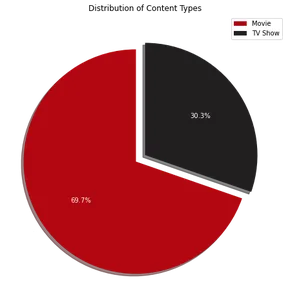
饼图可视化显示 Netflix 上大约 70% 的内容由电影组成,而其余 30% 是电视节目。 接下来,要确定 Netflix 最受欢迎的前 10 个国家/地区,我们可以使用以下代码:
Netflix 最受欢迎的 10 个国家
接下来,要确定 Netflix 最受欢迎的前 10 个国家/地区,我们可以使用以下代码:
# Remove white spaces from 'country' column
df_country['country'] = df_country['country'].str.rstrip() # Find value counts
country_counts = df_country['country'].value_counts() # Select the top 10 countries
top_10_countries = country_counts.head(10) # Plot the top 10 countries
plt.figure(figsize=(16, 10))
colors = ['#b20710'] + ['#221f1f'] * (len(top_10_countries) - 1)
bar_plot = sns.barplot(x=top_10_countries.index, y=top_10_countries.values, palette=colors) plt.xlabel('Country')
plt.ylabel('Number of Titles')
plt.title('Top 10 Countries Where Netflix is Popular') # Add count values on top of each bar
for index, value in enumerate(top_10_countries.values): bar_plot.text(index, value, str(value), ha='center', va='bottom') plt.show()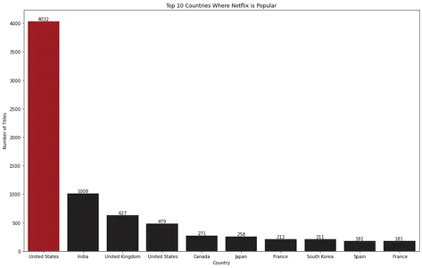
条形图可视化显示美国是 Netflix 最受欢迎的国家。
电影/电视节目数量排名前 10 位的演员
找出影视剧中出场次数最多的前10名演员,可以使用如下代码:
# Count the occurrences of each actor
cast_counts = df_cast['cast'].value_counts()[1:] # Select the top 10 actors
top_10_cast = cast_counts.head(10) plt.figure(figsize=(16, 8))
colors = ['#b20710'] + ['#221f1f'] * (len(top_10_cast) - 1)
bar_plot = sns.barplot(x=top_10_cast.index, y=top_10_cast.values, palette=colors) plt.xlabel('Actor')
plt.ylabel('Number of Appearances')
plt.title('Top 10 Actors by Movie/TV Show Count') # Add count values on top of each bar
for index, value in enumerate(top_10_cast.values): bar_plot.text(index, value, str(value), ha='center', va='bottom') plt.show()
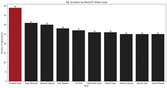
条形图显示 Anupam Kher 在电影和电视节目中的出场次数最多。
电影/电视节目数量排名前 10 位的导演
要确定执导电影或电视节目数量最多的前 10 位导演,您可以使用以下代码:
# Count the occurrences of each actor
director_counts = df_director['director'].value_counts()[1:] # Select the top 10 actors
top_10_directors = director_counts.head(10) plt.figure(figsize=(16, 8))
colors = ['#b20710'] + ['#221f1f'] * (len(top_10_directors) - 1)
bar_plot = sns.barplot(x=top_10_directors.index, y=top_10_directors.values, palette=colors) plt.xlabel('Director')
plt.ylabel('Number of Movies/TV Shows')
plt.title('Top 10 Directors by Movie/TV Show Count') # Add count values on top of each bar
for index, value in enumerate(top_10_directors.values): bar_plot.text(index, value, str(value), ha='center', va='bottom') plt.show()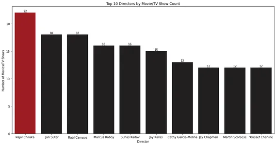
条形图显示电影或电视节目最多的前 10 名导演。 拉吉夫·奇拉卡 (Rajiv Chilaka) 似乎是 Netflix 库中导演最多的内容。
电影/电视节目数量排名前 10 的类别
要分析不同类别的内容分布,可以使用以下代码:
df_listed_in['listed_in'] = df_listed_in['listed_in'].str.strip() # Count the occurrences of each actor
listed_in_counts = df_listed_in['listed_in'].value_counts() # Select the top 10 actors
top_10_listed_in = listed_in_counts.head(10) plt.figure(figsize=(12, 8))
bar_plot = sns.barplot(x=top_10_listed_in.index, y=top_10_listed_in.values, palette=colors) # Customize the plot
plt.xlabel('Category')
plt.ylabel('Number of Movies/TV Shows')
plt.title('Top 10 Categories by Movie/TV Show Count')
plt.xticks(rotation=45) # Add count values on top of each bar
for index, value in enumerate(top_10_listed_in.values): bar_plot.text(index, value, str(value), ha='center', va='bottom') # Show the plot
plt.show()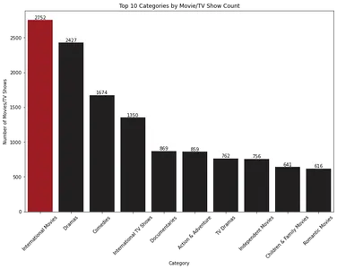
条形图根据数量显示电影和电视节目的前 10 个类别。 “国际电影”是最主要的类别,其次是“剧情片”。
随着时间的推移添加的电影和电视节目
要分析随着时间的推移增加的电影和电视节目,您可以使用以下代码:
# Filter the DataFrame to include only Movies and TV Shows
df_movies = df[df['type'] == 'Movie']
df_tv_shows = df[df['type'] == 'TV Show'] # Group the data by year and count the number of Movies and TV Shows # added in each year
movies_count = df_movies['year_added'].value_counts().sort_index()
tv_shows_count = df_tv_shows['year_added'].value_counts().sort_index() # Create a line chart to visualize the trends over time
plt.figure(figsize=(16, 8))
plt.plot(movies_count.index, movies_count.values, color='#b20710', label='Movies', linewidth=2)
plt.plot(tv_shows_count.index, tv_shows_count.values, color='#221f1f', label='TV Shows', linewidth=2) # Fill the area under the line charts
plt.fill_between(movies_count.index, movies_count.values, color='#b20710')
plt.fill_between(tv_shows_count.index, tv_shows_count.values, color='#221f1f') # Customize the plot
plt.xlabel('Year')
plt.ylabel('Count')
plt.title('Movies & TV Shows Added Over Time')
plt.legend() # Show the plot
plt.show()
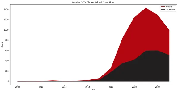
折线图说明了随着时间的推移添加到 Netflix 的电影和电视节目的数量。 它直观地表示了内容添加的增长和趋势,电影和电视节目有单独的线条。
Netflix 从 2015 年开始实现了真正的增长,我们可以看到这些年来它增加的电影多于电视节目。
此外,有趣的是,2020 年内容添加量有所下降。这可能是由于大流行情况所致。
接下来,我们探索不同月份的内容添加分布。 此分析有助于我们识别模式并了解 Netflix 何时推出新内容。
按月添加的内容
为了对此进行调查,我们从“date_added”列中提取月份并计算每个月的出现次数。 将此数据可视化为条形图,使我们能够快速识别内容添加量最高的月份。
# Extract the month from the 'date_added' column
df['month_added'] = pd.to_datetime(df['date_added']).dt.month_name() # Define the order of the months
month_order = ['January', 'February', 'March', 'April', 'May', 'June', 'July', 'August', 'September', 'October', 'November', 'December'] # Count the number of shows added in each month
monthly_counts = df['month_added'].value_counts().loc[month_order] # Determine the maximum count
max_count = monthly_counts.max() # Set the color for the highest bar and the rest of the bars
colors = ['#b20710' if count == max_count else '#221f1f' for count in monthly_counts] # Create the bar chart
plt.figure(figsize=(16, 8))
bar_plot = sns.barplot(x=monthly_counts.index, y=monthly_counts.values, palette=colors) # Customize the plot
plt.xlabel('Month')
plt.ylabel('Count')
plt.title('Content Added by Month') # Add count values on top of each bar
for index, value in enumerate(monthly_counts.values): bar_plot.text(index, value, str(value), ha='center', va='bottom') # Rotate x-axis labels for better readability
plt.xticks(rotation=45) # Show the plot
plt.show()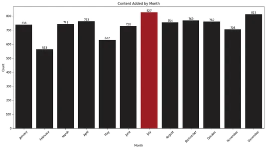
条形图显示 XNUMX 月和 XNUMX 月是 Netflix 向其库添加最多内容的月份。 对于希望在这几个月内期待新版本的观众来说,此信息可能很有价值。
Netflix 内容分析的另一个重要方面是了解收视率的分布。 通过检查每个评级类别的计数,我们可以确定平台上最流行的内容类型。
评级分布
我们首先计算每个评分类别的出现次数,并使用条形图将它们可视化。 这种可视化提供了评级分布的清晰概览。
# Count the occurrences of each rating
rating_counts = df['rating'].value_counts() # Create a bar chart to visualize the ratings
plt.figure(figsize=(16, 8))
colors = ['#b20710'] + ['#221f1f'] * (len(rating_counts) - 1)
sns.barplot(x=rating_counts.index, y=rating_counts.values, palette=colors) # Customize the plot
plt.xlabel('Rating')
plt.ylabel('Count')
plt.title('Distribution of Ratings') # Rotate x-axis labels for better readability
plt.xticks(rotation=45) # Show the plot
plt.show()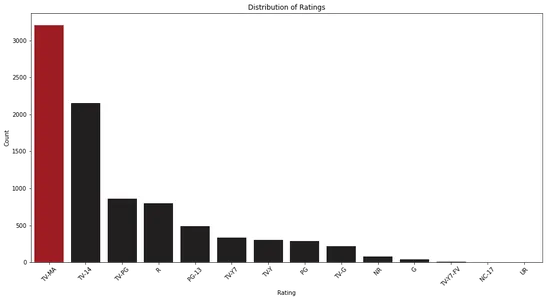
通过分析条形图,我们可以观察到 Netflix 的收视率分布。 它帮助我们确定最常见的评级类别及其相对频率。
类型相关热图
流派在 Netflix 上的内容分类和组织方面发挥着重要作用。 分析流派之间的相关性可以揭示不同类型内容之间有趣的关系。
我们创建了一个流派数据 DataFrame 来研究流派相关性并用零填充它。 通过迭代原始 DataFrame 中的每一行,我们根据列出的流派更新流派数据 DataFrame。 然后,我们使用该流派数据创建一个相关矩阵,并将其可视化为热图。
# Extracting unique genres from the 'listed_in' column
genres = df['listed_in'].str.split(', ', expand=True).stack().unique() # Create a new DataFrame to store the genre data
genre_data = pd.DataFrame(index=genres, columns=genres, dtype=float) # Fill the genre data DataFrame with zeros
genre_data.fillna(0, inplace=True) # Iterate over each row in the original DataFrame and update the genre data DataFrame
for _, row in df.iterrows(): listed_in = row['listed_in'].split(', ') for genre1 in listed_in: for genre2 in listed_in: genre_data.at[genre1, genre2] += 1 # Create a correlation matrix using the genre data
correlation_matrix = genre_data.corr() # Create the heatmap
plt.figure(figsize=(20, 16))
sns.heatmap(correlation_matrix, annot=False, cmap='coolwarm') # Customize the plot
plt.title('Genre Correlation Heatmap')
plt.xticks(rotation=90)
plt.yticks(rotation=0) # Show the plot
plt.show()
热图展示了不同类型之间的相关性。 通过分析热图,我们可以识别特定类型之间的强正相关,例如电视剧和国际电视节目、浪漫电视节目和国际电视节目。
电影长度和电视剧集数的分布
了解电影和电视节目的持续时间可以深入了解内容的长度,并帮助观众计划他们的观看时间。 通过检查电影长度和电视节目时长的分布,我们可以更好地了解 Netflix 上可用的内容。
为实现这一点,我们从“持续时间”列中提取电影长度和电视剧集数。 然后我们绘制直方图和箱线图来可视化电影长度和电视节目时长的分布。
# Extract the movie lengths and TV show episode counts
movie_lengths = df_movies['duration'].str.extract('(d+)', expand=False).astype(int)
tv_show_episodes = df_tv_shows['duration'].str.extract('(d+)', expand=False).astype(int) # Plot the histogram
plt.figure(figsize=(10, 6))
plt.hist(movie_lengths, bins=10, color='#b20710', label='Movies')
plt.hist(tv_show_episodes, bins=10, color='#221f1f', label='TV Shows') # Customize the plot
plt.xlabel('Duration/Episode Count')
plt.ylabel('Frequency')
plt.title('Distribution of Movie Lengths and TV Show Episode Counts')
plt.legend() # Show the plot
plt.show()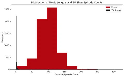
分析直方图,我们可以观察到 Netflix 上的大多数电影的时长都在 100 分钟左右。 另一方面,Netflix 上的大多数电视节目只有一季。
此外,通过检查箱线图,我们可以看到超过大约 2.5 小时的电影被视为异常值。 对于电视节目,找到超过四个季节的节目并不常见。
多年来电影/电视节目长度的趋势
我们可以绘制折线图来了解电影长度和电视节目集数多年来的变化情况。 通过分析这些趋势来识别内容持续时间的模式或变化。
我们首先从“持续时间”列中提取电影长度和电视节目集数。 然后,我们创建线图来可视化多年来电影长度和电视节目剧集的变化。
import seaborn as sns
import matplotlib.pyplot as plt # Extract the movie lengths and TV show episodes from the 'duration' column
movie_lengths = df_movies['duration'].str.extract('(d+)', expand=False).astype(int)
tv_show_episodes = df_tv_shows['duration'].str.extract('(d+)', expand=False).astype(int) # Create line plots for movie lengths and TV show episodes
plt.figure(figsize=(16, 8)) plt.subplot(2, 1, 1)
sns.lineplot(data=df_movies, x='release_year', y=movie_lengths, color=colors[0])
plt.xlabel('Release Year')
plt.ylabel('Movie Length')
plt.title('Trend of Movie Lengths Over the Years') plt.subplot(2, 1, 2)
sns.lineplot(data=df_tv_shows, x='release_year', y=tv_show_episodes,color=colors[1])
plt.xlabel('Release Year')
plt.ylabel('TV Show Episodes')
plt.title('Trend of TV Show Episodes Over the Years') # Adjust the layout and spacing
plt.tight_layout() # Show the plots
plt.show()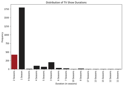
分析折线图,我们观察到令人兴奋的模式。 我们可以看到,电影长度开始增加,直到 1963-1964 年左右,然后逐渐下降,稳定在平均 100 分钟左右。 这表明随着时间的推移,观众的偏好发生了变化。
关于电视节目剧集,我们注意到自 2000 年代初以来一直存在的趋势,Netflix 上的大多数电视节目都有一到三季。 这表明观众更喜欢较短的系列或有限的系列格式。
标题和描述中最常用的词
分析标题和描述中最常用的词可以深入了解 Netflix 的主题和内容重点。 我们可以根据 Netflix 内容的标题和描述生成词云来揭示这些模式。
from wordcloud import WordCloud # Concatenate all the titles into a single string
text = ' '.join(df['title']) wordcloud = WordCloud(width = 800, height = 800, background_color ='white', min_font_size = 10).generate(text) # plot the WordCloud image
plt.figure(figsize = (8, 8), facecolor = None)
plt.imshow(wordcloud)
plt.axis("off")
plt.tight_layout(pad = 0) plt.show() # Concatenate all the titles into a single string
text = ' '.join(df['description']) wordcloud = WordCloud(width = 800, height = 800, background_color ='white', min_font_size = 10).generate(text) # plot the WordCloud image
plt.figure(figsize = (8, 8), facecolor = None)
plt.imshow(wordcloud)
plt.axis("off")
plt.tight_layout(pad = 0) plt.show()
检查标题的词云,我们观察到“爱情”、“女孩”、“男人”、“生活”和“世界”等词被频繁使用,表明存在浪漫、成年和戏剧Netflix 内容库中的流派。
分析用于描述的词云,我们注意到“生活”、“发现”和“家庭”等主要词,暗示了 Netflix 内容中普遍存在的个人旅程、人际关系和家庭动态等主题。
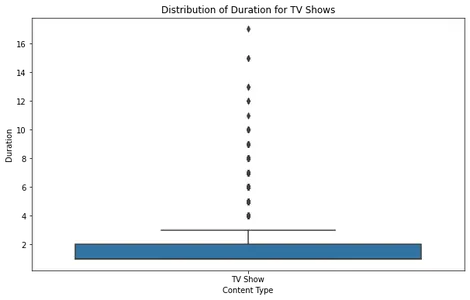
电影和电视节目的时长分布
通过分析电影和电视节目的时长分布,我们可以了解 Netflix 上可用内容的典型长度。 我们可以创建箱线图来可视化这些分布并识别异常值或标准持续时间。
# Extracting and converting the duration for movies
df_movies['duration'] = df_movies['duration'].str.extract('(d+)', expand=False).astype(int) # Creating a boxplot for movie duration
plt.figure(figsize=(10, 6))
sns.boxplot(data=df_movies, x='type', y='duration')
plt.xlabel('Content Type')
plt.ylabel('Duration')
plt.title('Distribution of Duration for Movies')
plt.show() # Extracting and converting the duration for TV shows
df_tv_shows['duration'] = df_tv_shows['duration'].str.extract('(d+)', expand=False).astype(int) # Creating a boxplot for TV show duration
plt.figure(figsize=(10, 6))
sns.boxplot(data=df_tv_shows, x='type', y='duration')
plt.xlabel('Content Type')
plt.ylabel('Duration')
plt.title('Distribution of Duration for TV Shows')
plt.show()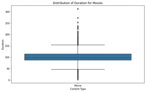
分析电影箱线图,我们可以看到大多数电影都在合理的持续时间范围内,很少有异常值超过大约 2.5 小时。 这表明 Netflix 上的大多数电影都设计为适合标准观看时间。
对于电视节目,箱线图显示大多数节目有 XNUMX 到 XNUMX 季,只有极少数异常值有更长的持续时间。 这与早期趋势一致,表明 Netflix 专注于较短的剧集格式。
结论
在这篇文章的帮助下,我们已经能够了解 -
- 数量:我们的分析显示,Netflix 添加的电影多于电视节目,符合电影在其内容库中占据主导地位的预期。
- 内容添加:XNUMX 月成为 Netflix 添加内容最多的月份,紧随其后的是 XNUMX 月,表明内容发布的战略方针。
- 类型相关性:在电视剧和国际电视节目、浪漫和国际电视节目以及独立电影和戏剧等各种类型之间观察到强烈的正相关。 这些相关性提供了对观众偏好和内容互连的洞察力。
- 电影时长:对电影时长的分析表明,在 1960 年代左右达到峰值,随后在 100 分钟左右稳定下来,突出了电影时长随时间变化的趋势。
- 电视节目剧集:Netflix 上的大多数电视节目都有一季,这表明观众更喜欢较短的剧集。
- 共同主题:爱情、生活、家庭和冒险等词经常出现在标题和描述中,捕捉了 Netflix 内容中反复出现的主题。
- 评级分布:多年来的评级分布提供了对不断变化的内容格局和观众接受度的洞察。
- 数据驱动的见解:我们的数据分析之旅展示了数据在揭开 Netflix 内容格局的奥秘方面的力量,为观众和内容创作者提供了宝贵的见解。
- 持续相关性:随着流媒体行业的发展,了解这些模式和趋势对于驾驭 Netflix 及其庞大的图书馆的动态景观变得越来越重要。
- 快乐流媒体:我们希望这个博客是进入 Netflix 世界的一次启迪和娱乐之旅,我们鼓励您在其不断变化的内容产品中探索迷人的故事。 让数据指导您的流媒体冒险!
官方文档和资源
请在下面找到我们分析中使用的库的官方链接。 您可以参考这些链接以获取有关这些库提供的方法和功能的更多信息:
- 熊猫: https://pandas.pydata.org/
- NumPy: https://numpy.org/
- Matplotlib: https://matplotlib.org/
- 科学派: https://scipy.org/
- Seaborn: https://seaborn.pydata.org/
本文中显示的媒体不属于 Analytics Vidhya 所有,其使用由作者自行决定。
相关
- SEO 支持的内容和 PR 分发。 今天得到放大。
- 柏拉图爱流。 Web3 数据智能。 知识放大。 访问这里。
- 与 Adryenn Ashley 一起铸造未来。 访问这里。
- 使用 PREIPO® 买卖 PRE-IPO 公司的股票。 访问这里。
- Sumber: https://www.analyticsvidhya.com/blog/2023/06/netflix-case-study-eda-unveiling-data-driven-strategies-for-streaming/
- :具有
- :是
- :不是
- :在哪里
- 1
- 10
- 100
- 12
- 20
- 2015
- 2020
- 2022
- 8
- 9
- a
- Able
- 关于
- 丰富
- 验收
- 访问
- 精准的
- 横过
- 演员
- 加
- 添加
- 增加
- 额外
- 增加
- 地址
- 添加
- 探险
- 瞄准
- 对齐
- 所有类型
- 允许
- 允许
- 聚敛
- 其中
- an
- 分析
- 分析
- 分析维迪亚
- 分析
- 分析
- 和
- 预料
- 任何
- 露面
- 的途径
- 约
- 四月
- 保健
- 国家 / 地区
- 围绕
- 刊文
- AS
- 方面
- 方面
- 协会
- At
- 属性
- 听众
- 八月
- 可用性
- 可使用
- 避免
- 背部
- 酒吧
- 酒吧
- 基地
- 基于
- BE
- 成为
- 成为
- 很
- 开始
- 开始
- 如下。
- 更好
- 之间
- 偏见
- 博客
- 半身裙/裤
- 盒子
- by
- 计算
- 计算
- CAN
- 能力
- 迷人
- 捕获
- 案件
- 案例研究
- 类别
- 分类
- 产品类别
- Center
- 更改
- 特点
- 图表
- 图表
- 检查
- 中国
- 选择
- 清除
- 密切
- 云端技术
- 码
- 采集
- 颜色
- 柱
- 列
- 相当常见
- 常用
- 公司
- 完成
- 全面
- 计算
- 考虑
- 一贯
- 由
- 消耗
- 内容
- 内容创作者
- 内容类型
- 转换
- 兑换
- 转换
- 相关
- 相关
- 可以
- 国家
- 国家
- 创建信息图
- 创建
- 创造
- 创作者
- 关键
- 定制
- data
- 数据分析
- 数据丢失
- 资料准备
- 数据科学
- 数据可视化
- 数据驱动
- 数据驱动策略
- 日期时间
- 十二月
- 深
- 演示
- 描述
- 描述
- 设计
- 详细
- 确定
- 偏差
- 不同
- 针对
- 副总经理
- 团队介绍
- 酌处权
- 显示
- 显示器
- 分配
- 分布
- 不同
- 多元化的观众
- 文件
- 优势
- 主宰
- 戏剧
- 下降
- 下降
- 删除
- 两
- 重复
- 为期
- ,我们将参加
- 动态
- 动力学
- 每
- 此前
- 早
- 生态系统
- 只
- 工作的影响。
- 其他
- 从事
- 出现
- enable
- 使
- 鼓励
- 提高
- 增强
- 确保
- 保证
- 娱乐
- 娱乐
- 爱好者
- 插曲
- 情节
- 必要
- 成熟
- 醚(ETH)
- 甚至
- 千变万化
- 所有的
- 进化
- 演变
- 演变
- 检查
- 令人兴奋的
- 排除
- 扩大
- 扩大
- 扩张
- 期望
- 有经验
- 勘探
- 探索
- 探讨
- 探索
- 提取
- 秋季
- 家庭
- 二月
- 少数
- 图
- 文件
- 填
- 电影
- 薄膜
- 过滤
- 找到最适合您的地方
- 寻找
- (名字)
- 适合
- 专注焦点
- 重点
- 其次
- 以下
- 针对
- 力
- 格式
- 发现
- 基金会
- 四
- 频率
- 频繁
- 新鲜
- 止
- 功能
- 功能
- 功能
- 进一步
- Gain增益
- 生成
- 得到
- 全球
- 全球业务
- 在全球范围内
- Go
- 渐渐
- 团队
- 事业发展
- 指南
- 民政事务总署
- 手
- 处理
- 处理
- 有
- 有
- 高度
- 帮助
- 帮助
- 相关信息
- 老旧房屋
- 最高
- 突出
- 阻碍
- 抱有希望
- HOURS
- 创新中心
- HTTPS
- ID
- 鉴定
- 确定
- if
- 说明
- 图片
- 影响力故事
- 进口
- 输入
- 有声有色
- in
- 包括
- 增加
- 日益
- 独立
- 指数
- 表示
- 表示
- 行业中的应用:
- 信息
- 初始
- 原来
- 可行的洞见
- 诚信
- 有趣
- 国际
- 成
- 奇妙
- 推出
- 调查
- 参与
- 问题
- IT
- 它的
- 一月
- 旅程
- 旅程
- 七月
- 六月
- 韩国
- 标签
- 景观
- 语言
- 层
- 布局
- 领导
- 学习用品
- 学习
- 长度
- Level
- 借力
- 库
- 自学资料库
- 生活
- 光
- 喜欢
- 有限
- Line
- 线
- 链接
- 已发布
- 加载
- 装载
- 不再
- 看
- 离
- 爱
- 机
- 机器学习
- 制成
- 保持
- 操作
- 三月
- matplotlib
- 矩阵
- 最多
- 可能..
- 意味着
- 媒体
- 方法
- 百万
- 大幅减低
- 最低限度
- 分钟
- 失踪
- 时尚
- 月
- 个月
- 更多
- 最先进的
- 电影
- 电影
- 姓名
- 导航
- 必要
- 打印车票
- Netflix公司
- 全新
- 下页
- 没有
- 北
- 北朝鲜
- 值得一提的
- 注意..
- 十一月
- 数
- 麻木
- 观察
- 获得
- 发生
- 十月
- of
- 折扣
- 提供
- 供品
- 优惠精选
- 官方
- on
- 一
- 仅由
- 运营
- or
- 秩序
- 组织
- 原版的
- 其他名称
- 我们的
- 超过
- 最划算
- 简介
- 拥有
- 垫
- 大熊猫
- 流感大流行
- 部分
- 模式
- 高峰
- 百分比
- 演出
- 个人
- 透视
- 计划
- 平台
- 平台
- 柏拉图
- 柏拉图数据智能
- 柏拉图数据
- 播放
- 热门
- 声望
- 积极
- 潜力
- 功率
- 喜好
- 准备
- 存在
- 流行
- 提供
- 提供
- 提供
- 优
- 公然
- 出版
- 季
- 很快
- 范围
- 等级
- 评分
- 准备
- 真实
- 合理
- 招待会
- 记录
- 经常性
- 关系
- 相对的
- 释放
- 发布
- 相关性
- 其余
- 卓越
- 去掉
- 更换
- 代表
- REST的
- 成果
- 揭示
- 揭密
- 揭示
- 革命性
- 右
- 角色
- 行
- 俄罗斯
- 科学
- 海生的
- 季节
- 季节性
- 季节
- 其次
- 第二季度
- 部分
- 看到
- 似乎
- 分开
- 另
- 九月
- 系列
- 集
- 转移
- 转移
- 显示
- 展示
- 展出
- 如图
- 作品
- 显著
- 自
- 单
- 情况
- So
- 一些
- 采购
- 剩余名额
- 具体的
- 分裂
- 标准
- 开始
- 开始
- 州
- 统计
- 步
- 步骤
- 商店
- 存储
- 故事
- 善用
- 战略方针
- 策略
- 策略
- 流
- 串
- 强烈
- 结构体
- 学习
- 字幕
- 顺利
- 这样
- 提示
- 适应性
- 概要
- 叙利亚
- 表
- 任务
- 条款
- 比
- 这
- 区域
- 世界
- 其
- 他们
- 然后
- 博曼
- 他们
- Free Introduction
- 那些
- 三
- 通过
- 次
- 标题
- 标题
- 标题
- 至
- 工具
- 最佳
- 返回顶部
- 改造
- 转型
- 转化
- 趋势
- 趋势
- tv
- 电视节目
- 类型
- 类型
- 普遍
- 罕见
- 揭露
- 下
- 强调
- 理解
- 理解
- 独特
- 联合的
- 美国
- 宇宙
- 直到
- 揭幕
- 更新
- us
- 使用
- 用过的
- 运用
- 有价值
- 有价值的信息
- 折扣值
- 价值观
- 各个
- 广阔
- 非常
- 观众
- 查看
- 可视化
- 想像
- 想
- 是
- 观看
- we
- 网页
- 为
- ,尤其是
- 而
- 白色
- WHO
- 广泛
- 将
- 中
- Word
- 话
- 世界
- 全世界
- X
- 年
- 年
- 您
- 您一站式解决方案
- 和风网