3D nanofabricated soft microrobots with super-compliant picoforce springs as onboard sensors and actuators – Nature Nanotechnology

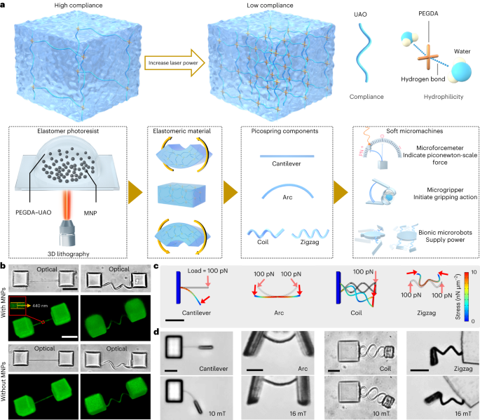
Magnetic-elastic photoresist preparation

All chemicals were purchased from Sigma-Aldrich unless otherwise specified. The elastic photoresist consisted of urethane acrylate oligomer 70 wt%, poly(ethylene glycol) diacrylate 28.40 wt% as the crosslinker, 1-(4-(2-(dimethylamino)ethoxy)phenyl)-2-phenyl-1-butanone 1.5 wt% as the photoinitiator, and a complex of 2,2,6,6-tetramethylpiperidine-1-oxyl 0.05 wt% and methyl methacrylate 0.05 wt% as the quencher. The mixture was bubbled with nitrogen for 30 min and vacuumed for 30 min to degas. MNPs were prepared based on a classic coprecipitation method. Briefly, 5.38 g FeCl₃·6H₂O and 1.98 g FeCl₂·4H₂O were dissolved in 200 ml H₂O. Then 7 ml 25% ammonium hydroxide was dropped in the mixture, which was continuously stirred for 3 h. The collected particles were then washed with water three times and further modified by 3-(trimethoxysilyl)propyl methacrylate in ethanol at concentrations of 1 wt% and 0.5 wt% at 80 °C for 1 h (ref. ²⁰). MNPs were collected after washing with ethanol three times. The magnetic-elastic photoresist was prepared by mixing MNPs into the elastic photoresist at a concentration of 5% or 10% for the special microturtle containing double concentration of MNPs. Finally, the magnetic-elastic photoresist was bubbled with N₂ for 30 min and vacuumed for 30 min. Prepared photoresist should be always kept from light at 4 °C before use.

Numerical analysis

To design the microstructures efficiently based on the material properties, simulations were performed to predict the shape morphing of the microstructures before fabrication. For the results presented in Figs. 1d and 6d, and Extended Data Figs. 3 and 7, we used a user-defined multiphysics module of the commercial finite element analysis software Comsol. All solids and fluids were regarded as incompressible. Young’s modulus E was set as 0.422 MPa for the microforcemeters and 1.525 Mpa for the other elastic components, according to mechanical characterization results of the cantilever picospring. The Poisson ratio for all materials was set as 0.49, assuming that the material is quasi-incompressible. In all simulations, the sperm medium (SP-TALP) was set as a Newtonian fluid with the density of 10³ kg m⁻³ and viscosity of 1 mPa s. During finite element analysis, the applied load was given as a function of the magnetic torque in the local coordinate system. The magnetic torque T^m was calculated by using a simplified function applied to the soft magnetic material⁵¹:

where θ is the angle from the magnetic field with a flux density of B to the easy magnetic axis of the segment; χ, V and μ represent the magnetic susceptibility and bulk volume of the segment, and the magnetic permeability of water (see details in Supplementary Text 2). The boundary loads of the mechanics simulation were applied parallel to the cross-section of the elastic springs in the local coordinate system. The magnetic torques applied on the flippers of the microturtle shown in Fig. 6d were calculated according to the equation above, by simplifying the flippers as rectangular shapes as projection in two dimensions.

The micropenguin was furthermore analysed with a kinematic model solved by the Runge–Kutta fourth-order iterative method with MATLAB. As shown in Extended Data Fig. 6d, the micropenguin flippers and torso were simplified as cuboids. The elastic components were simplified as linear springs. The bending stiffness of the elastic component was obtained by fitting the balanced magnetic torque with respect to the deflection angle, which is measured as half of the varied angle of two flippers at each magnetic field. Additional simulation parameters can be found in Supplementary Text 2. The simulation results were then used to guide the design and fabrication of the microstructures, and were furthermore validated by the experimental results.

Microstructure fabrication

Microstructures were fabricated by using a 3D direct laser writing system (Photonic Professional GT, Nanoscribe). During the fabrication, the laser power was set as 25.0 mW for all rigid parts, 5.5 mW for the force-sensing picosprings and 6.0 mW for all the other elastic components, unless otherwise specified. After exposure, the sample was developed in acetone for 24 h to remove all unpolymerized components. As shown in Extended Data Fig. 1a, the environment was changed from acetone to water-based media with pluronic acid F127 (PF127) as a thickener gradually at a rate of 200 μl min⁻¹ for 12 h. After that, the solution was gently replaced with SP-TALP by pipette. Structural integrality of the picospring-based microstructures was well kept after these operations (Extended Data Fig. 1b). Notably, in the microgripper experiment, SP-TALP was furthermore replaced by a cell media mimicking oviduct fluid (cell media containing 0.4% methylcellulose)⁵².

During the fabrication of the microoscillator, the coil-spring microoscillator and the microforcemeter, the glass substrate was silanized before use to avoid the detachment of the microstructures from the substrate. 3-(Trimethoxysilyl)propyl methacrylate was used to attach methacrylate terminal groups onto the substrate, forming a covalent linkage between the glass substrate and the magnetic-elastic photoresist⁵³.

During the fabrication of the microturtle, the exposure was performed twice by using the photoresist with and without MNPs. First, the elastic photoresist without MNPs was used to fabricate the torso. After that, the photoresist was replaced with magnetic-elastic photoresist. The glass substrate was glued with a glass capillary as an aligning indicator to be aligned to the previously marked tick lines on the sample holder to align the sample to the same position as the first exposure. The origin was found again based on the position of the fabricated torso and the structure code was corrected with a specific angle based on the orientation change of the torso to maximally enhance the fabrication accuracy. Then the second exposure was performed to fabricate the flippers and elastic components.

Material characterization

A confocal laser spectrum microscope (Zeiss LSM 980) was used to obtain the 3D geometry of the microforcemeter at excitation laser of 488 nm and emission detection of 580 nm. ImageJ was used to generate the 3D model of the structure and measure the dimensions.

The elastic property of the cantilever was calibrated by an optical trap system (Lumicks C-Trap). Five-micrometre polystyrene microbeads were used to calibrate the laser power of the optical trap, giving the trapping force constants of certain laser powers. Microbeads were then pulled to deform the microforcemeter as slowly as possible, so that the drag force could be neglected. The bending curve of the microforcemeter with respect to the applied force can then be determined by recording the positions of the microbead and the deflection angles of the cantilever (see details in Supplementary Text 1.2). Each group of measurements was repeated on three samples. Images and videos were analyzed with ImageJ and data were fitted with OriginPro. The viscosity of SP-TALP was taken as 1 mPa s. The mechanical characterization of the rigid parts fabricated at 25 mW was done using an AFM, shown in Supplementary Fig. 3 (see details in Supplementary Text 1.2).

The magnetization property of the material was characterized by a superconducting quantum interference device magnetometer (SQUID, Quantum Design) at room temperature with magnetic fields up to 100 mT. The samples were prepared as an array of 8,848 rectangular solids with a length of 15 μm and sectional area of 16 μm². The volume susceptibility was calculated as 0.1220, by fitting the magnetization with respect to the applied field using OriginPro software.

Propulsion force measurement by the microforcemeter

The sperm–motor microtubes, tubular microjets and microhelices were all fabricated by TPL using IP-DIP as photoresist. After exposure, the samples were dried in a critical point dryer after 20 min of development in mr-Dev 600 (Micro Resist) and washed three times with isopropanol. Metal layers of Fe (10 nm)/Ti (5 nm) were coated on the sperm–motor microtubes and the microhelices by sputtering. Layers of Fe (10 nm)/Ti (5 nm)/Pt (10 nm) were coated on the tubular microjet by e-beam deposition. Bovine sperm were prepared following the previously reported protocol². All samples were treated in PF127 solution (1%) for 0.5 h before use. The measurement of the sperm–motors was performed in the microforcemeter chamber with 1 ml SP-TALP containing about 10³ microtubes and 10⁴ sperm. The sperm–motor was formed when a sperm became constrained in a microtube by randomly swimming. The sperm–motor was then guided by the external magnetic field, at around 2 mT, towards the action bar of the microforcemeter. The magnetic field was adjusted perpendicularly to the action bar, to avoid the influence of the magnetic torque on the cantilever deformation. The measurement of the microjets was performed in SP-TALP containing 1% H₂O₂ and 0.1% sodium dodecyl sulfate. Approximately 20 microjets were added and guided in the same way as the sperm–motors. The measurement of the microhelices was performed by applying a rotating magnetic field of 10 mT at 40 Hz for magnetic actuation. The propulsion force, that is, the elastic force when the sperm–motor speed is zero, was calculated by linear interpolation in the calibration curve of the microforcemeter except for the propulsion force of the microjet, which was obtained from the finite element analysis simulation curve of the short microforcemeter. All measurements were done at 37 °C unless otherwise specified. Videos and data were analysed by ImageJ and OriginPro. Elastic forces were calculated by interpolation in the microforcemeter calibration curve in Fig. 3c,d.

Magnetic control of the microgripper

The magnetic actuation was performed by an electromagnet system (Magnebotix MFG 100-i). The time-sequential magnetic fields were generated by designing B_x, B_y and B_z with piecewise functions. After the media changing process, the microrobot and microgripper samples were treated in the ultrasonic bath for 5 min. Then a 100 μl pipette was used to gently blow the samples with media to fully detach the microstructures from the substrate without silanization. In the experiments of microrobots, the samples were then directly dispersed in SP-TALP and operated in the magnetic field. In the experiments of the microgripper, the sample solution was added with pre-prepared microobjects (microbeads and microclots). The microbead sample was obtained by directly dispersing 5 μm polystyrene microbeads at about 10³ ml⁻¹ as shown in Fig. 4c,f. The protein-based microclots were synthesized with bovine serum albumin by using a microemulsion method as reported previously². The oviduct-fluid-mimicking solution was prepared based on the HeLa cell media containing 0.4% methylcellulose to mimic the viscoelastic property of the fluid. Rotating magnetic fields were applied for the locomotion of the microgripper in a rolling manner and uniform magnetic fields were applied to open the gripper bucket. Videos and data were handled with ImageJ and OriginPro.

After manipulating the HeLa cells, the target cell was stained by a live/dead staining kit containing fluorescein diacetate and propidium iodide. Following a 10 min incubation period, multi-channel fluorescence images were captured using excitation at a wavelength of 470 nm for live cells (emission wavelength 530 nm) and 540 nm for dead cells (emission wavelength 618 nm). Subsequently, the target HeLa cell was cultured inside the microgripper’s bucket for an additional 4 h. A second manipulation was then performed to transport the HeLa cell along a rectangular trajectory. After this manipulation, fluorescence images were once again acquired. The presence of green fluorescence of the target cell after manipulation indicated that the microgripper had no adverse impact on the cell’s viability during manipulation, in contrast to the red fluorescence observed in randomly dead cells. The control of cell orientation shown in Fig. 4g was implemented by changing the direction of the applied magnetic field vector after the microgripper had gripped the cell cluster. A uniform magnetic field of 6 mT was applied along +x direction to grip and define the initial orientation of the cell cluster. For changing the cell orientation in the x–y (yaw) or x–z (pitch) planes, the magnetic field vectors were simply rotated along the z or y axes by any degree on demand. For changing the cell orientation in the y–z plane (roll), another rotating magnetic field at 2 mT and 20 Hz was applied. The orientation of the cell cluster in the y–z plane was changed by changing the rotation axis of the rotating magnetic field, while the uniform magnetic field of 6 mT was kept along the +x axis.

Magnetic control of the micropenguin and microturtle

Microrobots with time-symmetric motion cannot achieve a net displacement at low Reynolds number⁵⁴. An efficient strategy to break time symmetry is to make the microrobot’s orientation during morphing different from its orientation during recovery. As a demonstration, we implement an orientation-switching strategy to control the micropenguin. Extended Data Fig. 6a depicts the sequences of the magnetic fields with a cycle duration of 9 s as shown in Fig. 6a: 0–1 s, a uniform magnetic field of 16 mT was applied along the x axis (phases 1–2); 1–1.5 s, rotation magnetic field of 16 mT along the y axis; 1.5–2.5 s, uniform magnetic field of 2 mT along the z axis (phases 2–3); 2.5–4.5 s, rotation magnetic field of 2 mT along the y axis; 4.5–5.5 s, uniform magnetic field of 16 mT along the x axis (phases 3–4); 5.5–6 s, rotation magnetic field of 16 mT along the y axis; 6–7 s, uniform magnetic field of 2 mT along the z axis (phases 4–1); 7–9 s, rotation magnetic field of 2 mT along the y axis. After a cycle of 9 s, the micropenguin recovers its original orientation and gains a net displacement along the x axis. Extended Data Fig. 6b shows the magnetic field sequences with a cycle duration of 5.5 s of the micropenguin in a more efficient swimming manner. In this case, the uniform and rotation magnetic fields were mixed, enabling simultaneous micropenguin rotation and flipper opening and closing.

One disadvantage of the orientation-switching control strategy is the concomitant rotation of the whole robot, despite its universal applicability to elastic microrobots for generating a net displacement. This rotation can be avoided by using a set of picosprings driving different movable parts of microrobots with inhomogeneous magnetization, for example, the microturtle. Extended Data Fig. 7a shows the finite element analysis simulation results, which help seek out the most efficient directions of the magnetic fields. The magnetic field sequence of the final control strategy is shown in Extended Data Fig. 7b. Only uniform magnetic fields are needed to generate a net displacement for the microturtle owing to the coordinated actuation and buffering functions of the left and right pairs picosprings controlling different flippers. The microturtle was then only controlled to move in two dimensions of the x–y plane with no rotation or displacement in the z axis: 0–1 s, 2 mT along 15° (anticlockwise direction as positive) direction from the +y direction (symmetric axis of the microturtle); 1–1.5 s, 2 mT along −75° from +y; 1.5–2.5 s, 16 mT along −105° along +y; 2.5–3 s, 2 mT along +y. All locomotion experiments of the microrobots were performed in PBS at 25 °C. The microturtle contains double concentration of MNPs was controlled with a cycling period of 0.8 s (Extended Data Fig. 8) with comparable phase sections of 0–0.25 s, 0.25–0.4 s, 0.4–0.7 s and 0.7–0.8 s.

Biocompatibility evaluation

HeLa cells were used to assess the biocompatibility of the micromachines, specifically the microgripper arrays. In brief, 7 samples of fabricated microgripper arrays were placed in the cell culture wells of 6-well plates and filled with 3 ml of culture media. The control group wells were filled with only cell media. Each well was seeded with approximately 10⁵ HeLa cells. Following 48 h incubation, 1 well from the microgripper group and 1 from the control group were stained directly using the live/dead staining kit containing fluorescein diacetate (5 mg ml⁻¹ in acetone) and propidium iodide (1 mg ml⁻¹ in PBS). Multi-channel fluorescence images were taken using fluorescence microscopy (Cell Observer, Carl Zeiss Microscopy) under excitation at a wavelength of 470 nm for live cells (emission wavelength 530 nm) and 540 nm for dead cells (emission wavelength 618 nm). After 72 h incubation, the remaining 12 wells of cells were trypsinized, stained and counted under the fluorescence microscope. Cell viability was calculated as the ratio of the number of live cells (green) to the total cell count.

Statistics and reproducibility

No statistical method was used to predetermine the sample size. No data were excluded from the analyses. Cells and fabricated samples were randomly assigned to the respective groups before operation. The investigators were not blinded to allocation during experiments and outcome assessment.

Reporting summary

Further information on research design is available in the Nature Portfolio Reporting Summary linked to this article.

• SEO Powered Content & PR Distribution. Get Amplified Today.
• PlatoData.Network Vertical Generative Ai. Empower Yourself. Access Here.
• PlatoAiStream. Web3 Intelligence. Knowledge Amplified. Access Here.
• PlatoESG. Carbon, CleanTech, Energy, Environment, Solar, Waste Management. Access Here.
• PlatoHealth. Biotech and Clinical Trials Intelligence. Access Here.
• Source: https://www.nature.com/articles/s41565-023-01567-0