When learning about how to use Scikit-learn, we must obviously have an existing understanding of the underlying concepts of machine learning, as Scikit-learn is nothing more than a practical tool for implementing machine learning principles and related tasks. Machine learning is a subset of artificial intelligence that enables computers to learn and improve from experience without being explicitly programmed. The algorithms use training data to make predictions or decisions by uncovering patterns and insights. There are three main types of machine learning:
- Supervised learning – Models are trained on labeled data, learning to map inputs to outputs
- Unsupervised learning – Models work to uncover hidden patterns and groupings within unlabeled data
- Reinforcement learning – Models learn by interacting with an environment, receiving rewards and punishments to encourage optimal behavior
As you are undoubtedly aware, machine learning powers many aspects of modern society, generating enormous amounts of data. As data availability continues to grow, so does the importance of machine learning.
Scikit-learn is a popular open source Python library for machine learning. Some key reasons for its widespread use include:
- Simple and efficient tools for data analysis and modeling
- Accessible to Python programmers, with focus on clarity
- Built on NumPy, SciPy and matplotlib for easier integration
- Wide range of algorithms for tasks like classification, regression, clustering, dimensionality reduction
This tutorial aims to offer a step-by-step walkthrough of using Scikit-learn (mainly for common supervised learning tasks), focusing on getting started with extensive hands-on examples.
Installation and Setup
In order to install and use Scikit-learn, your system must have a functioning Python installation. We won’t be covering that here, but will assume that you have a functioning installation at this point.
Scikit-learn can be installed using pip, Python’s package manager:
pip install scikit-learnThis will also install any required dependencies like NumPy and SciPy. Once installed, Scikit-learn can be imported in your Python scripts as follows:
import sklearnTesting Your Installation
Once installed, you can start a Python interpreter and run the import command above.
Python 3.10.11 (main, May 2 2023, 00:28:57) [GCC 11.2.0] on linux
Type "help", "copyright", "credits" or "license" for more information.
>>> import sklearn
So long as you do not see any error messages, you are now ready to start using Scikit-learn!
Loading Sample Datasets
Scikit-learn provides a variety of sample datasets that we can use for testing and experimentation:
from sklearn import datasets iris = datasets.load_iris()
digits = datasets.load_digits()
The digits dataset contains images of handwritten digits along with their labels. We can start familiarizing ourselves with Scikit-learn using these sample datasets before moving on to real-world data.
Importance of Data Preprocessing
Real-world data is often incomplete, inconsistent, and contains errors. Data preprocessing transforms raw data into a usable format for machine learning, and is an essential step that can impact the performance of downstream models.
Many novice practitioners often overlook proper data preprocessing, instead jumping right into model training. However, low quality data inputs will lead to low quality models outputs, regardless of the sophistication of the algorithms used. Steps like properly handling missing data, detecting and removing outliers, feature encoding, and feature scaling help boost model accuracy.
Data preprocessing accounts for a major portion of the time and effort spent on machine learning projects. The old computer science adage “garbage in, garbage out” very much applies here. High quality data inputs are a prerequisite for high performance machine learning. The data preprocessing steps transform the raw data into a refined training set that allows the machine learning algorithms to effectively uncover predictive patterns and insights.
So in summary, properly preprocessing the data is an indispensable step in any machine learning workflow, and should receive substantial focus and diligent effort.
Loading and Understanding Data
Let’s load a sample dataset using Scikit-learn for demonstration:
from sklearn.datasets import load_iris
iris_data = load_iris()
We can explore the features and target values:
print(iris_data.data[0]) # Feature values for first sample
print(iris_data.target[0]) # Target value for first sample
We should understand the meaning of the features and target before proceeding.
Data Cleaning
Real data often contains missing, corrupt or outlier values. Scikit-learn provides tools to handle these issues:
from sklearn.impute import SimpleImputer imputer = SimpleImputer(strategy='mean') imputed_data = imputer.fit_transform(iris_data.data)The imputer replaces missing values with the mean, which is a common — but not the only — strategy. This is just one approach for data cleaning.
Feature Scaling
Algorithms like Support Vector Machines (SVMs) and neural networks are sensitive to the scale of input features. Inconsistent feature scales can result in these algorithms giving undue importance to features with larger scales, thereby affecting the model’s performance. Therefore, it’s essential to normalize or standardize the features to bring them onto a similar scale before training these algorithms.
from sklearn.preprocessing import StandardScaler scaler = StandardScaler()
scaled_data = scaler.fit_transform(iris_data.data)
StandardScaler standardizes features to have mean 0 and variance 1. Other scalers are also available.
Visualizing the Data
We can also visualize the data using matplotlib to gain further insights:
import matplotlib.pyplot as plt
plt.scatter(iris_data.data[:, 0], iris_data.data[:, 1], c=iris_data.target)
plt.xlabel('Sepal Length')
plt.ylabel('Sepal Width')
plt.show()
Data visualization serves multiple critical functions in the machine learning workflow. It allows you to spot underlying patterns and trends in the data, identify outliers that may skew model performance, and gain a deeper understanding of the relationships between variables. By visualizing the data beforehand, you can make more informed decisions during the feature selection and model training phases.
Overview of Scikit-learn Algorithms
Scikit-learn provides a variety of supervised and unsupervised algorithms:
- Classification: Logistic Regression, SVM, Naive Bayes, Decision Trees, Random Forest
- Regression: Linear Regression, SVR, Decision Trees, Random Forest
- Clustering: k-Means, DBSCAN, Agglomerative Clustering
Along with many others.
Choosing an Algorithm
Choosing the most appropriate machine learning algorithm is vital for building high quality models. The best algorithm depends on a number of key factors:
- The size and type of data available for training. Is it a small or large dataset? What kinds of features does it contain – images, text, numerical?
- The available computing resources. Algorithms differ in their computational complexity. Simple linear models train faster than deep neural networks.
- The specific problem we want to solve. Are we doing classification, regression, clustering, or something more complex?
- Any special requirements like the need for interpretability. Linear models are more interpretable than black-box methods.
- The desired accuracy/performance. Some algorithms simply perform better than others on certain tasks.
For our particular sample problem of categorizing iris flowers, a classification algorithm like Logistic Regression or Support Vector Machine would be most suitable. These can efficiently categorize the flowers based on the provided feature measurements. Other simpler algorithms may not provide sufficient accuracy. At the same time, very complex methods like deep neural networks would be overkill for this relatively simple dataset.
As we train models going forward, it is crucial to always select the most appropriate algorithms for our specific problems at hand, based on considerations such as those outlined above. Reliably choosing suitable algorithms will ensure we develop high quality machine learning systems.
Training a Simple Model
Let’s train a Logistic Regression model:
from sklearn.linear_model import LogisticRegression model = LogisticRegression()
model.fit(scaled_data, iris_data.target)
That’s it! The model is trained and ready for evaluation and use.
Training a More Complex Model
While simple linear models like logistic regression can often provide decent performance, for more complex datasets we may need to leverage more sophisticated algorithms. For example, ensemble methods combine multiple models together, using techniques like bagging and boosting, to improve overall predictive accuracy. As an illustration, we can train a random forest classifier, which aggregates many decision trees:
from sklearn.ensemble import RandomForestClassifier rf_model = RandomForestClassifier(n_estimators=100) rf_model.fit(scaled_data, iris_data.target)The random forest can capture non-linear relationships and complex interactions among the features, allowing it to produce more accurate predictions than any single decision tree. We can also employ algorithms like SVM, gradient boosted trees, and neural networks for further performance gains on challenging datasets. The key is to experiment with different algorithms beyond simple linear models to harness their strengths.
Note, however, that whether using a simple or more complex algorithm for model training, the Scikit-learn syntax allows for the same approach, reducing the learning curve dramatically. In fact, almost every task using the library can be expressed with the fit/transform/predict paradigm.
Importance of Evaluation
Evaluating a machine learning model’s performance is an absolutely crucial step before final deployment into production. Comprehensively evaluating models builds essential trust that the system will operate reliably once deployed. It also identifies potential areas needing improvement to enhance the model’s predictive accuracy and generalization ability. A model may appear highly accurate on the training data it was fit on, but still fail miserably on real-world data. This highlights the critical need to test models on held-out test sets and new data, not just the training data.
We must simulate how the model will perform once deployed. Rigorously evaluating models also provides insights into possible overfitting, where a model memorizes patterns in the training data but fails to learn generalizable relationships useful for out-of-sample prediction. Detecting overfitting prompts appropriate countermeasures like regularization and cross-validation. Evaluation further allows comparing multiple candidate models to select the best performing option. Models that do not provide sufficient lift over a simple benchmark model should potentially be re-engineered or replaced entirely.
In summary, comprehensively evaluating machine learning models is indispensable for ensuring they are dependable and adding value. It is not merely an optional analytic exercise, but an integral part of the model development workflow that enables deploying truly effective systems. So machine learning practitioners should devote substantial effort towards properly evaluating their models across relevant performance metrics on representative test sets before even considering deployment.
Train/Test Split
We split the data to evaluate model performance on new data:
from sklearn.model_selection import train_test_split X_train, X_test, y_train, y_test = train_test_split(scaled_data, iris_data.target)By convention, X refers to features and y refers to target variable. Please note that y_test and iris_data.target are different ways to refer to the same data.
Evaluation Metrics
For classification, key metrics include:
- Accuracy: Overall proportion of correct predictions
- Precision: Proportion of positive predictions that are actual positives
- Recall: Proportion of actual positives predicted positively
These can be computed via Scikit-learn’s classification report:
from sklearn.metrics import classification_report print(classification_report(y_test, model.predict(X_test)))This gives us insight into model performance.
Hyperparameter Tuning
Hyperparameters are model configuration settings. Tuning them can improve performance:
from sklearn.model_selection import GridSearchCV params = {'C': [0.1, 1, 10]}
grid_search = GridSearchCV(model, params, cv=5)
grid_search.fit(scaled_data, iris_data.target)
This grids over different regularization strengths to optimize model accuracy.
Cross-Validation
Cross-validation provides more reliable evaluation of hyperparameters:
from sklearn.model_selection import cross_val_score cross_val_scores = cross_val_score(model, scaled_data, iris_data.target, cv=5)It splits the data into 5 folds and evaluates performance on each.
Ensemble Methods
Combining multiple models can enhance performance. To demonstrate this, let’s first train a random forest model:
from sklearn.ensemble import RandomForestClassifier random_forest = RandomForestClassifier(n_estimators=100)
random_forest.fit(scaled_data, iris_data.target)
Now we can proceed to create an ensemble model using both our logistic regression and random forest models:
from sklearn.ensemble import VotingClassifier voting_clf = VotingClassifier(estimators=[('lr', model), ('rf', random_forest)])
voting_clf.fit(scaled_data, iris_data.target)
This ensemble model combines our previously trained logistic regression model, referred to as lr, with the newly defined random forest model, referred to as rf.
Model Stacking and Blending
More advanced ensemble techniques like stacking and blending build a meta-model to combine multiple base models. After training base models separately, a meta-model learns how best to combine them for optimal performance. This provides more flexibility than simple averaging or voting ensembles. The meta-learner can learn which models work best on different data segments. Stacking and blending ensembles with diverse base models often achieve state-of-the-art results across many machine learning tasks.
# Train base models
from sklearn.ensemble import RandomForestClassifier
from sklearn.svm import SVC rf = RandomForestClassifier()
svc = SVC() rf.fit(X_train, y_train)
svc.fit(X_train, y_train) # Make predictions to train meta-model
rf_predictions = rf.predict(X_test)
svc_predictions = svc.predict(X_test) # Create dataset for meta-model
blender = np.vstack((rf_predictions, svc_predictions)).T
blender_target = y_test # Fit meta-model on predictions
from sklearn.ensemble import GradientBoostingClassifier gb = GradientBoostingClassifier()
gb.fit(blender, blender_target) # Make final predictions
final_predictions = gb.predict(blender)
This trains a random forest and SVM model separately, then trains a gradient boosted tree on their predictions to produce the final output. The key steps are generating predictions from base models on the test set, then using those predictions as input features to train the meta-model.
Scikit-learn provides an extensive toolkit for machine learning with Python. In this tutorial, we covered the complete machine learning workflow using Scikit-learn — from installing the library and understanding its capabilities, to loading data, training models, evaluating model performance, tuning hyperparameters, and compiling ensembles. The library has become hugely popular due to its well-designed API, breadth of algorithms, and integration with the PyData stack. Sklearn empowers users to quickly and efficiently build models and generate predictions without getting bogged down in implementation details. With this solid foundation, you can now practically apply machine learning to real-world problems using Scikit-learn. The next step entails identifying issues that are amenable to ML techniques, and leveraging the skills from this tutorial to extract value.
Of course, there is always more to learn about Scikit-learn specifically and machine learning in general. The library implements cutting-edge algorithms like neural networks, manifold learning, and deep learning using its estimator API. You can always extend your competency by studying the theoretical workings of these methods. Scikit-learn also integrates with other Python libraries like Pandas for added data manipulation capabilities. Furthermore, a product like SageMaker provides a production platform for operationalizing Scikit-learn models at scale.
This tutorial is just the starting point — Scikit-learn is a versatile toolkit that will continue to serve your modeling needs as you take on more advanced challenges. The key is to continue practicing and honing your skills through hands-on projects. Practical experience with the full modeling lifecycle is the best teacher. With diligence and creativity, Scikit-learn provides the tools to unlock deep insights from all kinds of data.
Matthew Mayo (@mattmayo13) holds a Master’s degree in computer science and a graduate diploma in data mining. As Editor-in-Chief of KDnuggets, Matthew aims to make complex data science concepts accessible. His professional interests include natural language processing, machine learning algorithms, and exploring emerging AI. He is driven by a mission to democratize knowledge in the data science community. Matthew has been coding since he was 6 years old.
- SEO Powered Content & PR Distribution. Get Amplified Today.
- PlatoData.Network Vertical Generative Ai. Empower Yourself. Access Here.
- PlatoAiStream. Web3 Intelligence. Knowledge Amplified. Access Here.
- PlatoESG. Automotive / EVs, Carbon, CleanTech, Energy, Environment, Solar, Waste Management. Access Here.
- PlatoHealth. Biotech and Clinical Trials Intelligence. Access Here.
- ChartPrime. Elevate your Trading Game with ChartPrime. Access Here.
- BlockOffsets. Modernizing Environmental Offset Ownership. Access Here.
- Source: https://www.kdnuggets.com/5-steps-getting-started-scikit-learn?utm_source=rss&utm_medium=rss&utm_campaign=getting-started-with-scikit-learn-in-5-steps
- :has
- :is
- :not
- :where
- 1
- 10
- 11
- 12
- 13
- 14
- 2023
- 28
- 7
- 8
- 9
- a
- ability
- About
- above
- absolutely
- accessible
- Accounts
- accuracy
- accurate
- Achieve
- across
- actual
- added
- adding
- advanced
- affecting
- After
- AI
- aims
- algorithm
- algorithms
- All
- Allowing
- allows
- almost
- along
- also
- always
- among
- amounts
- an
- analysis
- Analytic
- and
- any
- api
- appear
- applies
- Apply
- approach
- appropriate
- ARE
- areas
- artificial
- artificial intelligence
- AS
- aspects
- assume
- At
- availability
- available
- averaging
- aware
- base
- based
- BE
- become
- been
- before
- being
- Benchmark
- BEST
- Better
- between
- Beyond
- Black-box
- Blender
- blending
- bogged
- boost
- Boosted
- boosting
- both
- breadth
- bring
- build
- Building
- builds
- but
- by
- CAN
- candidate
- capabilities
- capture
- categorizing
- certain
- challenges
- challenging
- choosing
- classification
- Cleaning
- clustering
- Coding
- combine
- combines
- Common
- community
- comparing
- complete
- complex
- complexity
- computer
- computer science
- computers
- computing
- concepts
- Configuration
- considerations
- considering
- contain
- contains
- continue
- continues
- Convention
- copyright
- correct
- course
- covered
- covering
- create
- creativity
- Credits
- critical
- crucial
- curve
- cutting-edge
- data
- data analysis
- data mining
- data science
- datasets
- decision
- decision tree
- decisions
- deep
- deep learning
- deep neural networks
- deeper
- defined
- Degree
- democratize
- demonstrate
- dependable
- dependencies
- depends
- deployed
- deploying
- deployment
- desired
- details
- develop
- Development
- differ
- different
- digits
- diligence
- diverse
- do
- does
- doing
- down
- dramatically
- driven
- due
- during
- each
- easier
- editor-in-chief
- Effective
- effectively
- efficient
- efficiently
- effort
- emerging
- empowers
- enables
- encourage
- enhance
- enormous
- ensure
- ensuring
- entirely
- Environment
- error
- Errors
- essential
- evaluate
- evaluating
- evaluation
- Even
- Every
- example
- examples
- Exercise
- existing
- experience
- experiment
- explore
- Exploring
- expressed
- extend
- extensive
- extract
- fact
- factors
- FAIL
- fails
- faster
- Feature
- Features
- final
- First
- fit
- Flexibility
- Focus
- focusing
- folds
- follows
- For
- forest
- format
- Forward
- Foundation
- from
- full
- functioning
- functions
- further
- Furthermore
- Gain
- Gains
- GCC
- General
- generate
- generating
- getting
- gives
- Giving
- going
- graduate
- Grow
- hand
- handle
- Handling
- hands-on
- harness
- Have
- he
- help
- here
- Hidden
- High
- highlights
- highly
- his
- holds
- How
- How To
- However
- HTTPS
- Hugely
- identifies
- identify
- identifying
- images
- Impact
- implementation
- implementing
- implements
- import
- importance
- improve
- improvement
- in
- include
- information
- informed
- input
- inputs
- insight
- insights
- install
- installation
- installed
- installing
- instead
- integral
- Integrates
- integration
- Intelligence
- interacting
- interactions
- interests
- into
- issues
- IT
- ITS
- just
- just one
- KDnuggets
- Key
- knowledge
- Labels
- language
- large
- larger
- lead
- LEARN
- learning
- Length
- let
- Leverage
- leveraging
- libraries
- Library
- License
- lifecycle
- like
- linux
- load
- loading
- Long
- Low
- machine
- machine learning
- Machines
- Main
- mainly
- major
- make
- manager
- Manipulation
- many
- map
- master
- matplotlib
- matthew
- May..
- mean
- meaning
- measurements
- merely
- messages
- methods
- Metrics
- Mining
- missing
- Mission
- ML
- ML techniques
- model
- modeling
- models
- Modern
- more
- most
- moving
- much
- multiple
- must
- Natural
- Natural Language
- Natural Language Processing
- Need
- needing
- needs
- networks
- Neural
- neural networks
- New
- newly
- next
- note
- nothing
- novice
- now
- number
- numpy
- of
- offer
- often
- Old
- on
- once
- ONE
- only
- onto
- open
- open source
- operate
- optimal
- Optimize
- Option
- or
- order
- Other
- Others
- our
- ourselves
- out
- outlier
- outlined
- output
- over
- overall
- package
- pandas
- paradigm
- part
- particular
- patterns
- perform
- performance
- performing
- platform
- plato
- Plato Data Intelligence
- PlatoData
- please
- Point
- Popular
- positive
- possible
- potential
- potentially
- powers
- Practical
- practically
- predicted
- prediction
- Predictions
- predictive
- previously
- principles
- Problem
- problems
- proceed
- processing
- produce
- Product
- Production
- professional
- programmed
- Programmers
- projects
- proper
- properly
- proportion
- provide
- provided
- provides
- Python
- quality
- quality data
- quickly
- random
- range
- Raw
- raw data
- ready
- real world
- reasons
- receive
- receiving
- reducing
- refer
- referred
- refers
- refined
- Regardless
- regression
- related
- Relationships
- relatively
- relevant
- reliable
- removing
- replaced
- report
- representative
- required
- Requirements
- Resources
- result
- Results
- Rewards
- right
- Run
- s
- sagemaker
- same
- Sample dataset
- Scale
- scales
- scaling
- Science
- scikit-learn
- scripts
- see
- segments
- selection
- sensitive
- separately
- serve
- serves
- set
- Sets
- settings
- should
- similar
- Simple
- simpler
- simply
- since
- single
- Size
- skew
- skills
- small
- So
- Society
- solid
- SOLVE
- some
- something
- sophisticated
- sophistication
- Source
- special
- specific
- specifically
- spent
- split
- Splits
- Spot
- stack
- stacking
- start
- started
- Starting
- state-of-the-art
- Step
- Steps
- Still
- Strategy
- strengths
- Studying
- substantial
- such
- sufficient
- suitable
- SUMMARY
- supervised learning
- support
- syntax
- system
- Systems
- T
- Take
- Target
- Task
- tasks
- teacher
- techniques
- test
- Testing
- text
- than
- that
- The
- their
- Them
- then
- theoretical
- There.
- thereby
- therefore
- These
- they
- this
- those
- three
- Through
- time
- to
- together
- tool
- toolkit
- tools
- towards
- Train
- trained
- Training
- trains
- Transform
- transforms
- tree
- Trees
- Trends
- truly
- Trust
- tutorial
- type
- types
- uncover
- underlying
- understand
- understanding
- undoubtedly
- unlock
- us
- usable
- use
- used
- users
- using
- value
- Values
- variable
- variables
- variety
- versatile
- very
- via
- visualization
- visualize
- vital
- Voting
- walkthrough
- want
- was
- ways
- we
- What
- whether
- which
- widespread
- will
- with
- within
- without
- Won
- Work
- workflow
- workings
- would
- X
- years
- you
- Your
- zephyrnet