How To Identify Missing Data In Time-Series Datasets

Republished By Plato

Followers: 0

Time-series data, collected nearly every second from a multiplicity of sources, is often subjected to several data quality issues, among which missing data.

In the context of sequential data, missing information can arise due to several reasons, namely errors occurring on acquisition systems (e.g. malfunction sensors), errors during the transmission process (e.g., faulty network connections), or errors during data collection (e.g., human error during data logging). These situations often generate sporadic and explicit missing values in our datasets, corresponding to small gaps in the stream of collected data.

Additionally, missing information can also arise naturally due to the characteristics of the domain itself, creating larger gaps in the data. For instance, a feature that stops being collected for a certain period of time, generating non-explicit missing data.

Regardless of the underlying cause, having missing data in our time-series sequences is highly prejudicial for forecasting and predictive modeling and may have serious consequences for both individuals (e.g., misguided risk assessment) and business outcomes (e.g., biased business decisions, loss of revenue and opportunities).

When preparing the data for modeling approaches, an important step is therefore being able to identify these patterns of unknown information, as they will help us decide on the best approach to handle the data efficiently and improve its consistency, either through some form of alignment correction, data interpolation, data imputation, or in some cases, casewise deletion (i.e., omit cases with missing values for a feature used in a particular analysis).

For that reason, performing a thorough exploratory data analysis and data profiling is indispensable not only to understand the data characteristics but also to make informed decisions on how to best prepare the data for analysis.

In this hands-on tutorial, we’ll explore how ydata-profiling can help us sort out these issues with the features recently introduced in the new release. We’ll be using the U.S. Pollution Dataset, available in Kaggle (License DbCL v1.0), that details information regarding NO2, O3, SO2, and CO pollutants across U.S. states.

To kickstart our tutorial, we first need to install the latest version of ydata-profiling:

pip install ydata-profiling==4.5.1

Then, we can load the data, remove unnecessary features, and focus on what we aim to investigate. For the purpose of this example, we will focus on the particular behavior of air pollutants’ measurements taken at the station of Arizona, Maricopa, Scottsdale:

import pandas as pd data = pd.read_csv("data/pollution_us_2000_2016.csv")
data = data.drop('Unnamed: 0', axis = 1) # dropping unnecessary index # Select data from Arizona, Maricopa, Scottsdale (Site Num: 3003)
data_scottsdale = data[data['Site Num'] == 3003].reset_index(drop=True)

Now, we’re ready to start profiling our dataset! Recall that, to use the time-series profiling, we need to pass the parameter tsmode=True so that ydata-profiling can identify time-dependent features:

# Change 'Data Local' to datetime
data_scottsdale['Date Local'] = pd.to_datetime(data_scottsdale['Date Local']) # Create the Profile Report
profile_scottsdale = ProfileReport(data_scottsdale, tsmode=True, sortby="Date Local")
profile_scottsdale.to_file('profile_scottsdale.html')

Time-Series Overview

The output report will be familiar to what we already know, but with an improved experience and new summary statistics for time-series data:

XXXXX

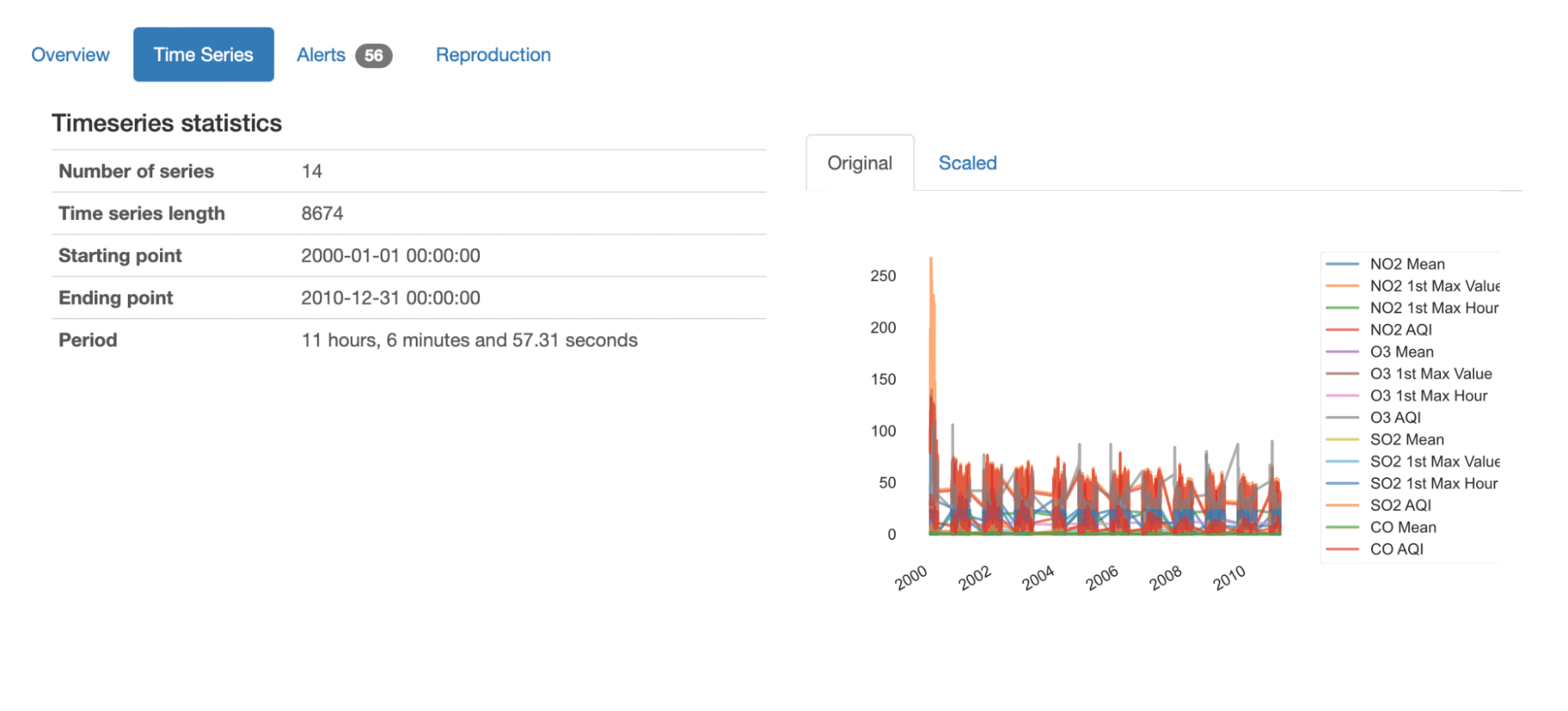
Immediately from the overview, we can get an overall understanding of this dataset by looking at the presented summary statistics:

It contains 14 different time-series, each with 8674 recorded values;
The dataset reports on 10 years of data from January 2000 to December 2010;
The average period of time sequences is 11 hours and (nearly) 7 minutes. This means that on average, we have measures being taken every 11 hours.

We can also get an overview plot of all series in data, either in their original or scaled values: we can easily grasp the overall variation of the sequences, as well as the components (NO2, O3, SO2, CO) and characteristics (Mean, 1st Max Value, 1st Max Hour, AQI) being measured.

Inspecting Missing Data

After having an overall view of the data, we can focus on the specifics of each time sequence.

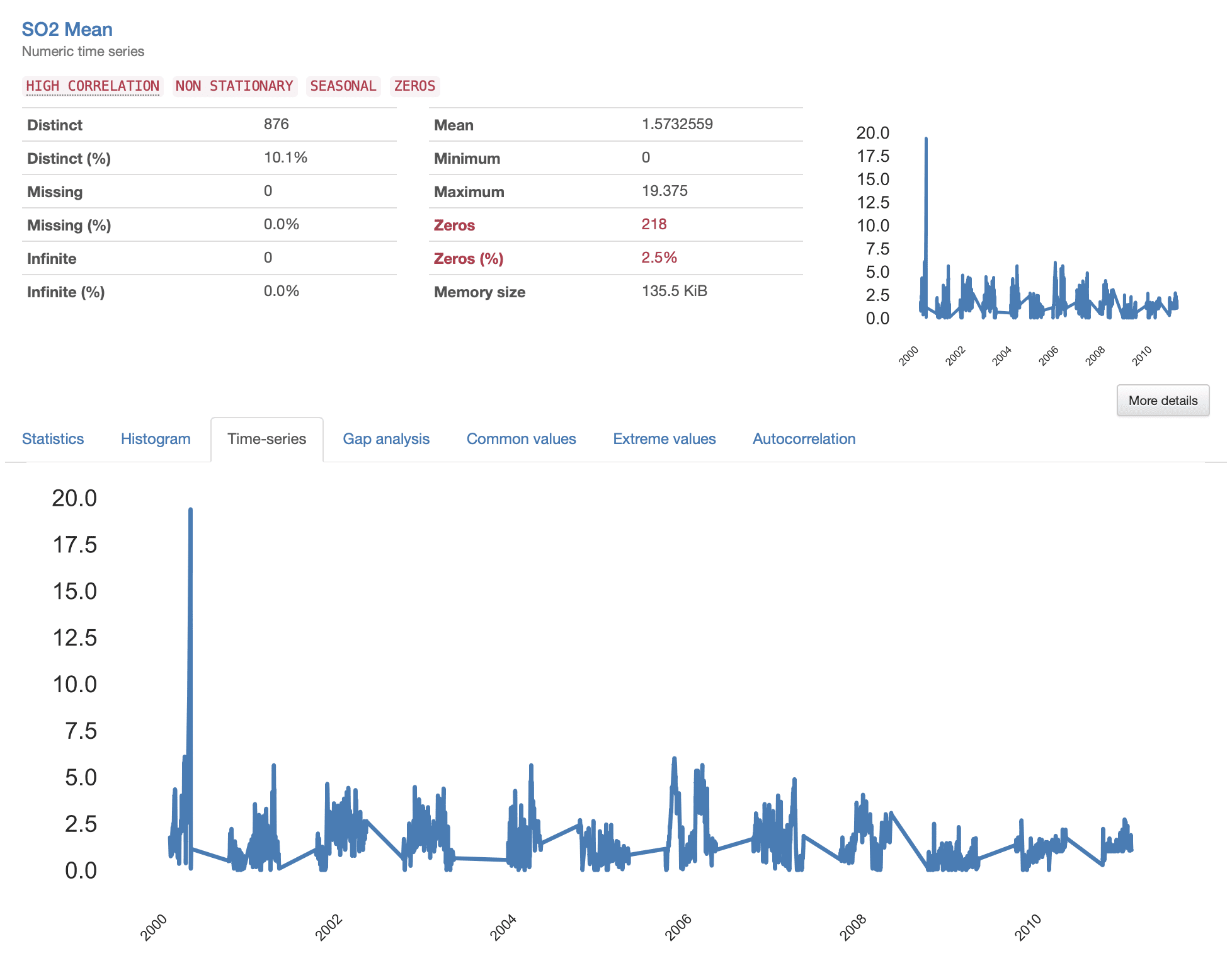
In the latest release of ydata-profiling, the profiling report was substantially improved with dedicated analysis for time-series data, namely reporting on the “Time Series” and “Gap Analysis”’ metrics. The identification of trends and missing patterns is extremely facilitated by these new features, where specific summary statistics and detailed visualizations are now available.

Something that stands out immediately is the flaky pattern that all time series present, where certain “jumps” seem to occur between consecutive measurements. This indicates the presence of missing data (“gaps” of missing information) that should be studied more closely. Let’s take a look at the S02 Mean as an example.

XXXXX

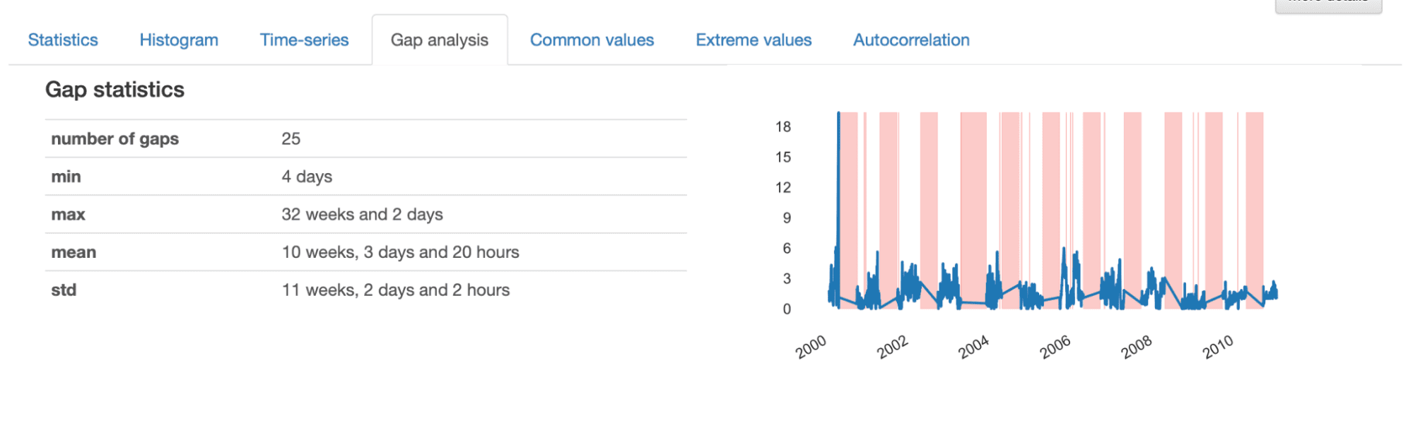
When investigating the details given in the Gap Analysis, we get an informative description of the characteristics of the identified gaps. Overall, there are 25 gaps in the time-series, with a minimum length of 4 days, a maximum of 32 weeks, and an average of 10 weeks.

From the visualization presented, we note somewhat “random” gaps represented by thinner stripes, and larger gaps which seem to follow a repetitive pattern. This indicates that we seem to have two different patterns of missing data in our dataset.

Smaller gaps correspond to sporadic events generating missing data, most likely occurring due to errors in the acquisition process, and can often be easily interpolated or deleted from the dataset. In turn, larger gaps are more complex and need to be analyzed in more detail, as they may reveal an underlying pattern that needs to be addressed more thoroughly.

In our example, if we were to investigate the larger gaps, we would in fact discover that they reflect a seasonal pattern:

df = data_scottsdale.copy()
for year in df["Date Local"].dt.year.unique(): for month in range(1,13): if ((df["Date Local"].dt.year == year) & (df["Date Local"].dt.month ==month)).sum() == 0: print(f'Year {year} is missing month {month}.')

# Year 2000 is missing month 4.
# Year 2000 is missing month 5.
# Year 2000 is missing month 6.
# Year 2000 is missing month 7.
# Year 2000 is missing month 8.
# (...)
# Year 2007 is missing month 5.
# Year 2007 is missing month 6.
# Year 2007 is missing month 7.
# Year 2007 is missing month 8.
# (...)
# Year 2010 is missing month 5.
# Year 2010 is missing month 6.
# Year 2010 is missing month 7.
# Year 2010 is missing month 8.

As suspected, the time-series presents some large information gaps that seem to be repetitive, even seasonal: in most years, the data was not collected between May to August (months 5 to 8). This may have occurred due to unpredictable reasons, or known business decisions, for example, related to cutting costs, or simply related to seasonal variations of pollutants associated with weather patterns, temperature, humidity, and atmospheric conditions.

Based on these findings, we could then investigate why this happened, if something should be done to prevent it in the future, and how to handle the data we currently have.

Throughout this tutorial, we’ve seen how important it is to understand the patterns of missing data in time-series and how an effective profiling can reveal the mysteries behind gaps of missing information. From telecom, healthcare, energy, and finance, all sectors collecting time-series data will face missing data at some point and will need to decide the best way to handle and extract all possible knowledge from them.

With a comprehensive data profiling, we can make an informed and efficient decision depending on the data characteristics at hand:

Gaps of information can be caused by sporadic events that derive from errors in acquisition, transmission, and collection. We can fix the issue to prevent it from happening again and interpolate or impute the missing gaps, depending on the length of the gap;
Gaps of information can also represent seasonal or repeated patterns. We may choose to restructure our pipeline to start collecting the missing information or replace the missing gaps with external information from other distributed systems. We can also identify if the process of retrieval was unsuccessful (maybe a fat-finger query on the data engineering side, we all have those days!).

I hope this tutorial has shed some light on how to identify and characterize missing data in your time-series data appropriately and I can’t wait to see what you’ll find in your own gap analysis! Drop me a line in the comments for any questions or suggestions or find me at the Data-Centric AI Community!

Fabiana Clemente is cofounder and CDO of YData, combining data understanding, causality, and privacy as her main fields of work and research, with the mission of making data actionable for organizations. As an enthusiastic data practitioner she hosts the podcast When Machine Learning Meets Privacy and is a guest speaker on the Datacast and Privacy Please podcasts. She also speaks at conferences such as ODSC and PyData.