Monk’s Disease Detective: Guide to AI-Powered Plant Health

Introduction

Agriculture is the lifeblood of our civilization, providing sustenance and nourishment to billions around the globe. However, this vital industry faces a relentless adversary: plant diseases. These microscopic threats can wreak havoc on crops, leading to significant economic losses and food shortages. The key to safeguarding our agricultural heritage lies in early detection and timely intervention, where cutting-edge technology steps in. This comprehensive guide will embark on a journey into plant disease classification using Monk, a powerful machine-learning library. By the end of this article, you’ll be equipped with the knowledge to harness the potential of artificial intelligence in identifying and combating plant diseases effectively.

So, fasten your seatbelts as we explore how Monk empowers us to create, train, and optimize deep learning models for plant disease classification. But before we dive into the technical aspects, let’s set up the stage by understanding the significance of this endeavor and why Monk plays a pivotal role.

Learning Objectives

• Understand the fundamentals of the Monk software/library.
• Learn how to install and set up Monk on your local machine or preferred development environment.
• Explore the importance of high-quality data in machine learning.
• Learn how to acquire, preprocess, and organize plant disease image datasets for classification tasks using Monk.
• Gain insights into selecting appropriate deep-learning model architectures for plant disease classification.
• Understand how to configure and fine-tune models within Monk, including pre-trained models for transfer learning.

This article was published as a part of the Data Science Blogathon.

Hands-On Guide: Creating Your First Disease Classifier with Monk

This section will walk you through the step-by-step process of building your Monk model for plant disease classification. Whether you’re new to machine learning or a seasoned data scientist, follow these instructions to get started on your plant disease classification journey.

Step 1: Data Collection

In this first step, we will gather the necessary dataset for our plant disease classification project. Follow these steps to collect the data:

The fantastic team at Plant Village gathered the dataset

1. Upload Kaggle API Token:

• Use the following code to upload your Kaggle API token. This token is required to download datasets from Kaggle.

from google.colab import files
files.upload()

2. Install the Kaggle Python Package:

• You must install the Kaggle Python package to interact with Kaggle from your Colab environment. Run the following command:

!pip install kaggle

3. Set Kaggle Configuration Directory:

• Set the Kaggle configuration directory to “/content” using the following code:

import os
os.environ['KAGGLE_CONFIG_DIR'] = '/content'

4. Set Appropriate Permissions:

• Ensure that the Kaggle API token file has the correct permissions by running:

!chmod 600 /content/kaggle.json

5. Download the Dataset:

• Use the Kaggle API to download the plant disease dataset by running this command:

!kaggle datasets download -d "prashantmalge/plant-disease"

6. Unzip the Dataset:

• Finally, unzip the downloaded dataset using the following command:

!unzip plant-disease.zip

This will make the dataset available in your Colab environment for further processing and training. Adjust the dataset name and paths as needed for your specific project.

Step 2: Setting Up Monk

First, you must set up Monk on your local machine or cloud environment. Follow these steps to get Monk up and running:

1. Clone the Monk repository:

# Clone the Monk repository
!git clone https://github.com/Tessellate-Imaging/monk_v1.git # Add the Monk repository to the Python path
import sys
sys.path.append("./monk_v1/monk") # Install any required packages or dependencies if needed
# Uncomment and add your installation command here
# !pip install -r /kaggle/working/monk_v1/installation/requirements_kaggle.txt

2. Install Monk using pip:

!pip install -U monk-colab

Step 3: Create an Experiment

Now, let’s create a Monk experiment. An experiment is a structured environment where you define the parameters and configurations for training your disease classifier. Here’s a code snippet to get you started:

from pytorch_prototype import prototype # Create an experiment
ptf = prototype(verbose=1)
ptf.Prototype("plant_disease", "exp1")

In this code, we’ve named our experiment “plant_disease” with the tag “exp1.” You can adjust the names according to your project.

Step 4: Data Loading and Preprocessing

Load your dataset and apply data transforms for preprocessing. Monk provides convenient functions for loading data and using transforms. Here’s an example:

# Load the dataset and define transforms
ptf.Default(dataset_path=["./dataset/train", "./dataset/val"], model_name="resnet18", freeze_base_network=True, num_epochs=5)

In this snippet, we specify the dataset path and the model architecture (ResNet-18) and freeze the base network’s weights.

Step 5: Quick Model Finder

Choose a model architecture that suits your needs and initiate the training process. Monk supports various pre-trained models, and you can fine-tune them as required. Here’s how you can do it:

# Analysis - 1 # Analysis Project Name
analysis_name = "Model_Finder"; # Models to analyse
# First element in the list- Model Name
# Second element in the list - Boolean value to freeze base network or not
# Third element in the list - Boolean value to use pretrained model as the starting point or not
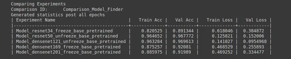
models = [["resnet34", True, True], ["resnet50", False, True], ["densenet121", False, True], ["densenet169", True, True], ["densenet201", True, True]]; # Num epochs for each experiment to run epochs=5; # Percentage of original dataset to take in for experimentation
percent_data=10; # "keep_all" - Keep all the sub experiments created
# "keep_non" - Delete all sub experiments created
ptf.Analyse_Models(analysis_name, models, percent_data, num_epochs=epochs, state="keep_none"); 

1. Analysis Project Name: analysis_name is a variable that stores the name of the analysis project. In this case, it’s set to “Model_Finder.”
2. Models to Analyze: The models list specifies the models you want to analyze. Each model is represented as a list with three elements:
3. Num Epochs: the number of epochs you want to run each experiment for. In this case, it’s set to 5.
4. Percentage of Original Dataset: percent_data specifies the percentage of the original dataset to use for experimentation. It’s set to 10%, meaning only 10% of the dataset will be used.
5. State: The state parameter determines whether to keep or delete sub-experiments. When set to “keep_none,” sub-experiments will not be kept, and only the final results will be retained.
6. Analyse_Models: Finally, the ptf.Analyse_Models() function is called with the specified parameters to perform the model analysis. It will run experiments for each model and record the results.

This code is helpful for quickly testing multiple models with different configurations to find the best-performing model for your task. Selecting an appropriate model architecture is a standard step in machine learning and deep learning projects.

Output : 

Step 6: Update The Model

## Update Model Architecture
ptf.update_model_name("densenet121");
ptf.update_freeze_base_network(True);
ptf.update_use_pretrained(True);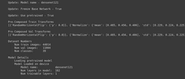
ptf.Reload();

1. Update Model Name: ptf.update_model_name(“densenet121”) updates the model architecture to “densenet121.” This means that you are switching from the previously used model to DenseNet-121.
2. Update Freeze Base Network: ptf.update_freeze_base_network(True) sets the flag to freeze the base network to “True.” Freezing the base network means that the pre-trained layers of the model will not be updated during training. They will remain fixed, and only the additional layers (if any) will be trained. This can be useful when using pre-trained models for transfer learning.
3. Update Use Pretrained: ptf.update_use_pretrained(True) sets the flag to use pre-trained weights to “True.” This indicates that you want to initialize the model with pre-trained weights. Using pre-trained weights as a starting point for transfer learning is common, especially when you switch to a new model architecture like DenseNet-121.
4. Reload: ptf.Reload() reloads the model with the updated configurations. After changing the model architecture and its settings, reloading the model to apply these changes is essential.

In summary, this code switches the model architecture to DenseNet-121, freezes the base network, and uses pre-trained weights. These changes are then applied to the model by reloading it.

Output : 

Step 7: Find the Right Batch Size

#Analysis - 2 # Analysis Project Name
analysis_name = "Batch_Size_Finder"; # Batch sizes to explore
batch_sizes = [4, 8, 16, 32]; # Num epochs for each experiment to run epochs = 10; # Percentage of original dataset to take in for experimentation
percent_data = 10; # "keep_all" - Keep all the sub experiments created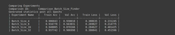
# "keep_non" - Delete all sub experiments created ptf.Analyse_Batch_Sizes(analysis_name, batch_sizes, percent_data, num_epochs=epochs, state="keep_none"); 

1. Analysis Name: analysis_name = “Batch_Size_Finder” defines the name of your analysis, which is “Batch_Size_Finder” in this case. This name helps you identify the purpose of this analysis.
2. Batch Sizes to Explore: batch_sizes = [4, 8, 16, 32] lists different batch sizes you want to explore during the analysis. In this example, you consider batch sizes 4, 8, 16, and 32.
3. Num Epochs: epochs = 10 specifies the number of training epochs for each experiment during the analysis. Each experiment will run for ten epochs to evaluate the model’s performance with different batch sizes.
4. Percentage of Original Dataset: percent_data = 10 defines the percentage of the original dataset you want to use for experimentation. In this case, you are using 10% of the dataset.
5. State: state=”keep_none” specifies the state of sub-experiments created during the analysis. In this case, “keep_none” means you do not want to keep any sub-experiments created during this analysis. They will be deleted after the study is completed.
6. Analyse Batch Sizes: ptf.Analyse_Batch_Sizes(analysis_name, batch_sizes, percent_data, num_epochs=epochs, state=”keep_none”) initiates the batch size analysis. This function will run experiments with different batch sizes (4, 8, 16, and 32) to evaluate their impact on model performance.

This analysis aims to determine the batch size that results in the best training and validation performance for your deep learning model. Different batch sizes can affect training speed and convergence; this analysis helps you find an optimal value.

Output : 

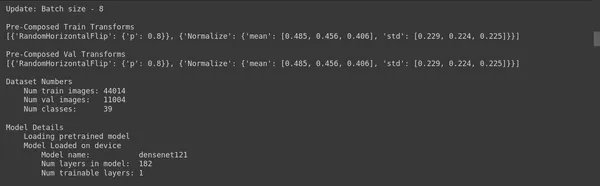
Step 8: Update Batch Size

## Update Batch Size
ptf.update_batch_size(8);
ptf.Reload();

1. Update Batch Size: ptf.update_batch_size(8) updates the batch size of your model to 8. This means your model will process data in batches of size eight samples during training. Batch size is a hyperparameter that can influence your model’s training speed, memory usage, and convergence.
2. Reload: ptf.Reload() reloads the model with the updated batch size. This is necessary because changing the batch size can affect the memory requirements of your model, and reloading ensures that the model is configured correctly with the new batch size.

Setting the batch size to 8 means that your model should process data in 8 samples per batch during training. This value was determined from your batch size analysis (as shown in the previous code snippet) to find an optimal batch size for your specific deep-learning task.

Output : 

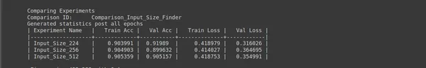
Step 9: Find the Correct Input Dimension

#Analysis - 3 # Analysis Project Name
analysis_name = "Input_Size_Finder"; # Input sizes to explore input_sizes = [224, 256, 512]; # Num epochs for each experiment to run epochs=5; # Percentage of original dataset to take in for experimentation
percent_data=10; # "keep_all" - Keep all the sub experiments created
# "keep_non" - Delete all sub experiments created ptf.Analyse_Input_Sizes(analysis_name, input_sizes, percent_data, num_epochs=epochs, state="keep_none"); 

1. Analysis Project Name: analysis_name = “Input_Size_Finder” defines a name for this analysis project used to organize and label the experiments related to input size.
2. Input Sizes to Explore: input_sizes = [224, 256, 512] specifies a list of input sizes (image dimensions) you want to explore. You are testing three different input sizes: 224×224, 256×256, and 512×512 pixels.
3. Num Epochs: epochs = five sets the number of training epochs for each experiment. In this case, you train the model for five epochs for each input size.
4. Percentage of Original Dataset: percent_data = 10 specifies the percentage of the original dataset to use for experimentation. Using a smaller portion of the dataset can help speed up the analysis while providing insights into how different input sizes affect model performance.
5. State: state=”keep_none” indicates that you want to keep only the best-performing experiment and discard others. This is useful for efficiently identifying the optimal input size without cluttering your workspace with multiple experiments.

This analysis lets you determine which input size works best for your specific deep-learning task. Different input sizes can impact model performance and training speed, so finding the right balance for your project is essential.

Output : 

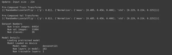
Step 10: Update Input Size

## Update Input Size ptf.update_input_size(224);
ptf.Reload();

1. Update Input Size: ptf.update_input_size(224) sets the input size of your model to 224×224 pixels. This means that your model will expect input images to have dimensions of 224 pixels in width and 224 pixels in height. Changing the input size can significantly impact your model’s performance and training time.
2. Reload: ptf.Reload() reloads the model with the updated input size. This step is necessary because changing the input size requires modifications to the model architecture. Reloading ensures that the model is correctly configured with the new input size.

By setting the input size to 224×224 pixels, you have effectively prepared your model to accept images of this size during training and inference. The choice of input size should align with your dataset and task requirements, and it’s often a critical hyperparameter to tune for optimal results.

Output : 

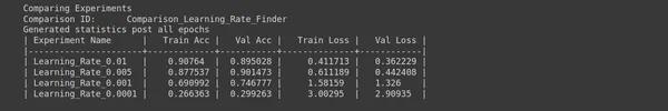
Step 11: Find Out the Correct Starting LR

#Analysis - 4 # Analysis Project Name
analysis_name = "Learning_Rate_Finder" # Learning rates to explore
lrs = [0.01, 0.005, 0.001, 0.0001]; # Num epochs for each experiment to run
epochs=5 # Percentage of original dataset to take in for experimentation
percent_data=10 # "keep_all" - Keep all the sub experiments created
# "keep_non" - Delete all sub experiments created
ptf.Analyse_Learning_Rates(analysis_name, lrs, percent_data, num_epochs=epochs, state="keep_none"); 

1. Analysis Project Name: analysis_name = “Learning_Rate_Finder” sets the name of your learning rate analysis project. You will use this name to organize the results of your experiments.
2. Learning Rates to Explore: lrs = [0.01, 0.005, 0.001, 0.0001] specifies a list of learning rates to explore during the analysis. Learning rate is a crucial hyperparameter in training deep neural networks, and finding the correct learning rate can significantly impact training success.
3. Num Epochs: epochs = 5 determines the number of epochs (training iterations) to run for each learning rate experiment. This helps assess how quickly the model converges with different learning rates.
4. Percentage of Original Dataset: percent_data = 10 defines the percentage of your original dataset used for experimentation. Using a smaller subset of the data can speed up the analysis process while still providing insights.
5. “keep_all” or “keep_none”: state=”keep_none” specifies whether to keep or delete all sub-experiments created during the learning rate analysis. In this case, “keep_none” means that sub-experiments will not be saved, likely because the primary goal is to identify the best learning rate rather than keep the intermediate results.

After running this code, the analysis will explore the specified learning rates, train the model for a few epochs with each learning rate, and collect performance metrics. This information will help you choose your model and dataset’s most suitable learning rate.

Output : 

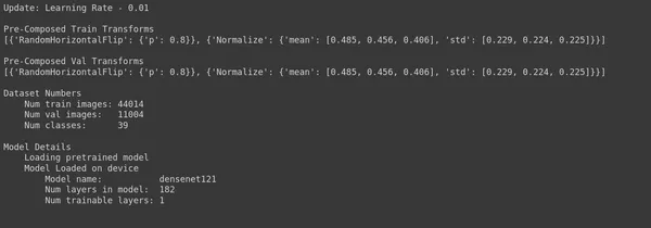
Step 12: Update LR

## Update Learning Rate
ptf.update_learning_rate(0.01);
ptf.Reload();

1. Update Learning Rate: ptf.update_learning_rate(0.01) updates the learning rate to 0.01. The learning rate is a hyperparameter that controls the step size during optimization. It determines how much the model’s parameters are updated during each training iteration.
2. Reload: ptf.Reload() reloads the model with the updated learning rate. Reloading the model ensures that your changes to the learning rate take effect during the subsequent training sessions.

Setting the learning rate to 0.01 allows you to specify a new learning rate for your model. Adjusting the learning rate is common in fine-tuning deep learning models to improve training stability and convergence.

Output : 

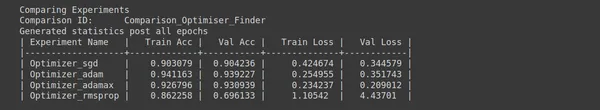
Step 13: Optimiser Hunting

# Analysis - 5
# Analysis Project Name
analysis_name = "Optimiser_Finder"; # Optimizers to explore
optimizers = ["sgd", "adam", "adamax", "rmsprop"]; #Model name, learning rate # Num epochs for each experiment to run epochs = 5; # Percentage of original dataset to take in for experimentation
percent_data = 10; # "keep_all" - Keep all the sub experiments created
# "keep_non" - Delete all sub experiments created
ptf.Analyse_Optimizers(analysis_name, optimizers, percent_data, num_epochs=epochs, state="keep_none"); 

1. Analysis Project Name: analysis_name = “Optimiser_Finder”; defines the name of the analysis project as “Optimiser_Finder.” This project will focus on finding the optimal optimizer for your model.
2. Optimizers to Explore: An optimizer is a list that contains the names of optimizers to be explored. The optimizers include “sgd,” “adam,” “adamax,” and “rmsprop.” Each optimizer has its own set of optimization techniques and hyperparameters.
3. Num Epochs: epochs = 5; specifies the number of epochs for each experiment run during the analysis. An epoch is one complete pass through the entire training dataset.
4. Percentage of Original Dataset: percent_data = 10; determines the percentage of the original dataset to use for experimentation. In this case, 10% of the dataset will be used.
5. Analyse_Optimizers: ptf.Analyse_Optimizers(analysis_name, optimizers, percent_data, num_epochs=epochs, state=”keep_none”); initiates the analysis of different optimizers. It will run experiments using each optimizer listed in the optimizers list and record the results.

By analyzing different optimizers, you can identify which works best for your dataset and deep learning model. The choice of optimizer can significantly impact the training and performance of your neural network.

Output : 

Step 14: Update Optimiser

## Update Optimiser ptf.optimizer_adamax(0.001);
ptf.Reload();

1. Update Optimizer Name: ptf.optimizer_adamax(0.001); set the optimizer to “Adamax” with a learning rate of 0.001.
2. Reload Model: ptf.Reload(); reloads the model with the new optimizer configuration.

You are changing the optimization algorithm used during training by updating the optimizer to “Adamax” with a specific learning rate. Different optimizers may converge at different rates, leading to variations in the training process and final model performance. It’s common to experiment with other optimizers and learning rates to find the best combination for your specific deep-learning task.

Step 15: Set Intermediate State- Saving To False

ptf.update_save_intermediate_models(False);

• ptf: Refers to the PyTorch Prototype object you’ve created.
• update_save_intermediate_models(False): This function updates the setting for saving intermediate models during training. You turn off the option to save intermediate models by passing False as the argument.

Intermediate models are snapshots of your model’s parameters saved at specific intervals during training. They can help resume training from a particular checkpoint or analyze the model’s performance at various stages of training.

Setting this option to False means that your code will not save intermediate models during the training process, which can be beneficial if you want to conserve disk space or do not need to keep track of intermediate checkpoints.

Next, we create a new experiment using ‘copy_experiment’ and resume training to achieve further improvement.

ptf = prototype(verbose=1);
ptf.Prototype("plant_disease", "exp2", copy_from=["plant_disease", "exp1"]);

1. ptf = prototype(verbose=1);: You create a new Prototype object named ptf with verbose mode enabled. This object allows you to define and manage machine learning experiments.
2. ptf.Prototype(“plant_disease”, “exp2”, copy_from=[“plant_disease”, “exp1”]);: This line specifies the details of the new experiment:

By creating a new experiment with the same settings as an existing one, you can quickly iterate on your experiments while maintaining consistency in configurations and tracking progress.

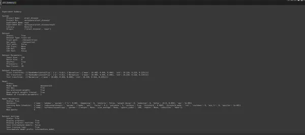
Summary of the experiment configuration:

ptf.Summary()

Output :

Step 16: Compare

Monk provides a streamlined “Compare” function that gathers statistics, visualizes results, and helps users decide which model architectures and hyperparameters are most effective. This step aids in the iterative process of fine-tuning models and progressively improving their performance, ultimately guiding the selection of the best-performing model configurations for deployment.

from compare_prototype import compare
ctf = compare(verbose=1);
ctf.Comparison("plant_disease");
ctf.Add_Experiment("plant_disease", "exp1");
ctf.Add_Experiment("plant_disease", "exp2");

These code snippets demonstrate the use of Monk’s “compare_prototype” module. First, it imports the necessary “compare” function. Then, it initializes a comparison object “ctf” with verbosity set to 1 for reporting. The comparison is named “plant_disease” using ctf.Comparison.

Following this, two experiments, “exp1” and “exp2,” conducted under the project “plant_disease,” are added to the comparison using ctf.Add_Experiment. This allows users to analyze and compare these two experiments’ results, metrics, and performance to make informed decisions about model selection and fine-tuning.

Step 17: Inference

Inference in Monk uses a trained model to predict new, unseen data. It allows you to utilize your trained model for real-world applications, such as classifying images, recognizing objects, or making decisions based on the model’s output. Inference typically involves loading a trained model, providing input data, and obtaining predictions or classifications from the model. Monk offers tools and functions to streamline the inference process and simplify deploying machine-learning models for practical use.

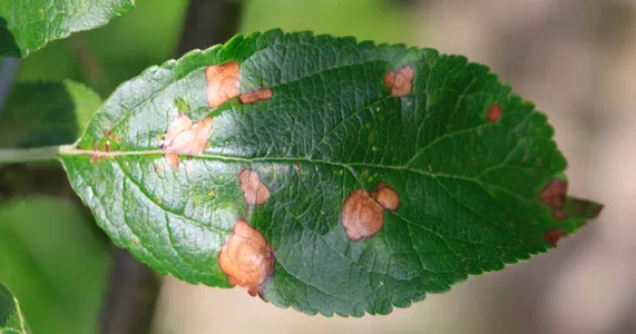
import numpy as np
import PIL.Image as Image
import requests test_url = "https://gardenerspath.com/wp-content/uploads/2019/08/ Frogeye-spots-Botryosphaeria-obtusa-on-apple-leaf-FB.jpg" # URL of the image to be downloaded is defined as image_url r = requests.get(test_url) # create HTTP response object with open('test.jpg','wb') as f: f.write(r.content) test = Image.open('./test.jpg')
test

Output :

ptf.Prototype("plant_disease", "exp2", eval_infer=True);

• ptf.Prototype(“plant_disease”, “exp2”, eval_infer=True);: This line sets up a new experiment named “exp2” under the project “plant_disease” using Monk’s Prototype function. It also enables evaluation and inference mode (eval_infer=True), indicating that this experiment will be used for making predictions on new data.

Output :

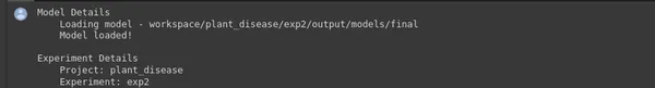
1. Model Details: After initializing the experiment, the code loads a pre-trained model. In this case, it’s loading a model from the directory “workspace/plant_disease/exp2/output/models/final.” This model will be used for inference.
2. Experiment Details: This section provides information about the experiment, including the project name (“plant_disease”), experiment name (“exp2”), and the directory where the experiment is stored

Step 18: Prediction

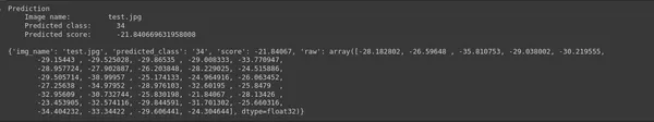
img_name = "test.jpg";
predictions = ptf.Infer(img_name=img_name, return_raw=True);
print(predictions)

1. img_name = “test.jpg”;: This line specifies the name of the image file (“test.jpg”) that you want to perform inference on. You can replace “test.jpg” with the path to the image you want to analyze.
2. Predictions = ptf.Infer(img_name=img_name, return_raw=True);: This line of code calls the “Infer” function provided by Monk’s experiment (ptf) to make predictions on the specified image. It inputs the image file name and requests raw prediction scores by setting “return_raw=True.” This means it will return the raw numerical scores for each class.
3. print(predictions): Finally, the code prints out the predictions. These predictions typically include information such as the predicted class and associated raw scores for each class.

This code allows you to analyze the specified image using the trained model and obtain predictions for various classes and their confidence scores. The printed output will provide insights into the model’s prediction for the given image.

import csv def read_labels(): mydict = {} with open('./dataset/labels.csv', mode='r') as infile: reader = csv.reader(infile) with open('labels_new.csv', mode='w') as outfile: writer = csv.writer(outfile) mydict = {rows[0]:rows[1] for rows in reader} return mydict def predict_label(predictions): pred_class = predictions['predicted_class'] label_dict = read_labels() out_label = label_dict[pred_class] return out_label print("Predicted class for test image is : {}".format(predict_label(predictions)))

1. read_labels() Function: This function reads label information from the “labels.csv” file. It opens the CSV file, reads its contents, and creates a dictionary (mydict) where keys are class IDs and values are the corresponding labels. It then writes this label information to a new CSV file called “labels_new.csv.”
2. predict_label(predictions) Function: This function takes the predictions obtained from the previous inference as input. It extracts the predicted class ID from the predictions and uses the label dictionary created earlier to find the corresponding label. The label is then returned as out_label.
3. Printing the Result: The code calls the predict_label(predictions) function to obtain the label associated with the predicted class and prints it as the “Predicted class for the test image is.”

In summary, this code helps you translate the numeric class ID predicted by the model into a human-readable label, making it easier to understand the model’s output.

Output: Predicted class for test image is: Apple___Black_rot

Advanced Techniques for Plant Disease Classification

Let’s explore advanced techniques and strategies to take your plant disease classification project to the next level.

1. Transfer Learning with Custom Data

While using pre-trained models is an excellent starting point, you can further improve your classifier’s accuracy by fine-tuning it with custom data. Collect more images specific to your target plant species and diseases. You can adapt a pre-trained model on your dataset by fine-tuning it to recognize unique patterns and symptoms.

# Fine-tuning a pre-trained model with custom data
ptf.update_model_name("resnet50")
ptf.update_freeze_base_network(False) # Unfreeze base network for fine-tuning
ptf.update_use_pretrained(True)
ptf.Reload()
ptf.Train()

2. Data Augmentation

Data augmentation is a powerful technique to increase the diversity of your training dataset artificially. By applying random transformations such as rotation, cropping, and brightness adjustments to your images, you can enhance your model’s ability to generalize. Monk provides convenient functions for data augmentation:

# Apply data augmentation transforms
ptf.apply_random_rotation(train=True, val=True)
ptf.apply_random_crop(scale=[0.8, 1.0], ratio=[0.8, 1.2], train=True)
ptf.apply_random_brightness(train=True)

3. Handling Class Imbalance

In real-world scenarios, you may encounter class imbalance, where some plant diseases are more prevalent than others. To address this, consider techniques like oversampling minority classes or applying class weights during training. Monk offers class-weighted loss functions to handle imbalanced datasets.

# Use a class-weighted loss function
ptf.loss_weighted_softmax_crossentropy(class_weights)

4. Ensemble Learning

Ensemble learning involves combining predictions from multiple models to improve accuracy and robustness. You can create an ensemble of different architectures or variations of the same model to achieve better results. Monk supports ensemble learning, allowing you to experiment with different combinations of models.

# Create an ensemble of models
ensemble = ptf.create_ensemble(models)
ensemble.Train()

5. Hyperparameter Tuning

Fine-tuning hyperparameters is crucial for optimizing your model’s performance. Monk provides tools for hyperparameter tuning, allowing you to explore various learning rates, batch sizes, and optimization algorithms.

# Hyperparameter tuning - Learning rate, batch size, optimizer
ptf.Analyse_Learning_Rates("LR_Finder", lrs, percent_data=10, num_epochs=5)
ptf.Analyse_Batch_Sizes("Batch_Size_Finder", batch_sizes, percent_data=10, num_epochs=5)
ptf.Analyse_Optimizers("Optimizer_Finder", optimizers, percent_data=10, num_epochs=5)

6. Model Interpretability

Understanding why a model makes specific predictions is essential, especially in critical applications like disease classification. Monk provides interpretability tools like Grad-CAM (Gradient-weighted Class Activation Mapping) to visualize which regions of an image are most influential for a prediction.

# Visualize model predictions with Grad-CAM
heatmap = ptf.Visualize_With_GradCAM(image_path, target_layer)

Conclusion

In this comprehensive guide, we’ve explored the fascinating world of plant disease classification using Monk. We’ve covered everything from setting up your experiments to fine-tuning models and understanding real-world applications. As we conclude, let’s recap the key takeaways and discuss the exciting future directions of this technology.

Key Takeaways: 

1. Monk Simplifies Deep Learning: Monk provides a user-friendly and intuitive interface for building, training, and deploying deep learning models. Its modular approach allows even beginners to dive into computer vision effortlessly.
2. Early Disease Detection: Plant diseases can devastate crops and threaten food security. Monk-powered models enable early disease detection, helping farmers proactively protect their crops.
3. Precision Agriculture: Monk contributes to precision agriculture by optimizing resource usage, reducing chemical inputs, and increasing crop yields. Farmers can achieve higher profitability and environmental sustainability.
4. Real-World Impact: Monk’s applications extend beyond agriculture to research, conservation, and citizen science. It empowers individuals and organizations to impact plant health and ecosystems positively.

Resources for Further Learning

To dive deeper into plant disease classification with Monk, here are some valuable resources:

• Monk Official Documentation -> Docs
• Plant Village Dataset -> Docs
• Monk setup -> Docs
• Quick Mode PyTorch -> Docs
• Quick Mode Keras -> Docs
• Quick Mode Gluon -> Docs
• Model Finder -> Docs

Monk remains at the forefront for plant disease classification solutions. Its user-friendly interface and powerful capabilities empower individuals and organizations to contribute to the well-being of our planet’s ecosystems and the global food supply.

Frequently Asked Questions

The media shown in this article is not owned by Analytics Vidhya and is used at the Author’s discretion.

Related

• SEO Powered Content & PR Distribution. Get Amplified Today.
• PlatoData.Network Vertical Generative Ai. Empower Yourself. Access Here.
• PlatoAiStream. Web3 Intelligence. Knowledge Amplified. Access Here.
• PlatoESG. Carbon, CleanTech, Energy, Environment, Solar, Waste Management. Access Here.
• PlatoHealth. Biotech and Clinical Trials Intelligence. Access Here.
• Source: https://www.analyticsvidhya.com/blog/2023/10/monk-for-plant-disease-classification/