Sentiment Analysis In Python: Going Beyond Bag Of Words

Republished By Plato

Followers: 0

Sentiment Analysis in Python: Going Beyond Bag of Words
Image created on DALL-E

Do you know that election results can be predicted to some extent by doing sentiment analysis? Data science can be both amusing and very useful when applied to real-life situations rather than working with mock datasets.

In this article, we will conduct a brief case study using Twitter data. In the end, you will see a case study that has a significant impact on real life, which will surely pique your interest. But first, let’s start with the basics.

Sentiment analysis is a method, used to predict feelings, like digital psychologists. With this, psychologist you created, the destiny of the text you’ll analyze will be in your hands. You can do it like the famous psychologist Freud, or you can just be there like a psychologist, charging 10 dollars per session.

Just like your psychologist listens and understands your emotions, sentiment analysis does the same things on text, like reviews, comments, or tweets, as we will do in the next section. To do that, let’s start doing a case study on the ready dataset.

To do sentiment analysis, we will use datasets from Kaggle. Here this dataset was collected by using twitter api. Here is the link to this dataset: https://www.kaggle.com/datasets/kazanova/sentiment140

Now, let’s start exploring the dataset.

Explore Dataset

Now, before doing sentiment analysis, let’s explore our dataset. To read it, use encoding. Because of this, we will add column names afterwards. You can increase the methods to do data exploration. Head, info, and describe method will give you a great heads up; let’s see the code.

import pandas as pd data = pd.read_csv('training.csv', encoding='ISO-8859-1', header=None)
column_names = ['target', 'ids', 'date', 'flag', 'user', 'text']
data.columns = column_names
head = data.head()
info = data.info()
describe = data.describe()
head, info, describe

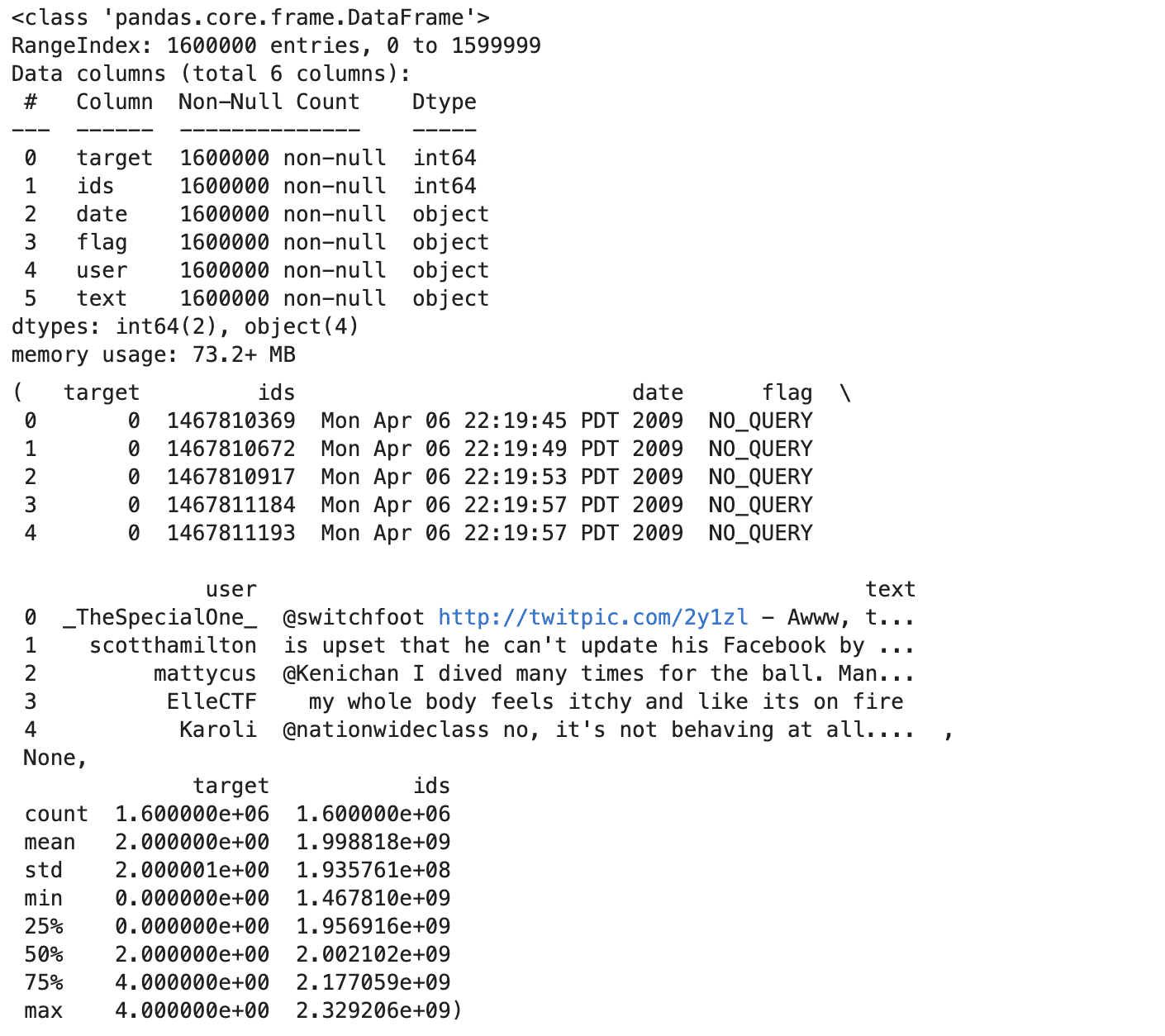
Here is the output.

Sentiment Analysis in Python: Going Beyond Bag of Words

Of course, you can run these methods one by one if you don’t have image limit on your project. Let’s see the insights we collect from these exploration methods above.

Insights

The dataset has 1.6 million tweets, with no missing values in any column.
Each tweet has a target sentiment (0 for negative,2 neutral, 4 for positive), an ID, a timestamp, a flag (query or ‘NO_QUERY’), the username, and the text.
The sentiment targets are balanced, with an equal number of positive and negative labels.

Visualize the Dataset

Wonderful, we have both statistical and structural knowledge about our dataset. Now, let’s create some visualizations to picture it. Now, we all know the sharpest sentiments, positive and negative. To see which words will be using for that, we will be using one of the python libraries called wordcloud.

This library will visualize your datasets according to the frequency of the words in it. If words are used frequently, you will understand it by looking at their size of it, there is a positive relation, if the word is bigger, it should be used a lot.

But first, we should select positive and negative tweets and combine them together by using python join method afterwards. Let’s see the code.

# Separate positive and negative tweets based on the 'target' column
positive_tweets = data[data['target'] == 4]['text']
negative_tweets = data[data['target'] == 0]['text'] # Sample some positive and negative tweets to create word clouds
sample_positive_text = " ".join(text for text in positive_tweets.sample(frac=0.1, random_state=23))
sample_negative_text = " ".join(text for text in negative_tweets.sample(frac=0.1, random_state=23)) # Generate word cloud images for both positive and negative sentiments
wordcloud_positive = WordCloud(width=800, height=400, max_words=200, background_color="white").generate(sample_positive_text)
wordcloud_negative = WordCloud(width=800, height=400, max_words=200, background_color="white").generate(sample_negative_text) # Display the generated image using matplotlib
plt.figure(figsize=(15, 7.5)) # Positive word cloud
plt.subplot(1, 2, 1)
plt.imshow(wordcloud_positive, interpolation='bilinear')
plt.title('Positive Tweets Word Cloud')
plt.axis("off") # Negative word cloud
plt.subplot(1, 2, 2)
plt.imshow(wordcloud_negative, interpolation='bilinear')
plt.title('Negative Tweets Word Cloud')
plt.axis("off") plt.show()

Here is the output.

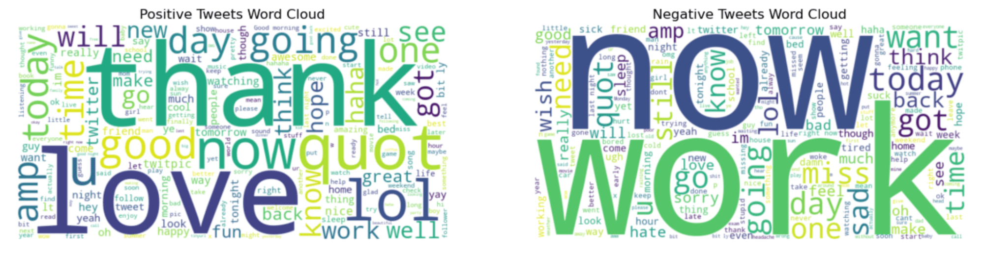
Sentiment Analysis in Python: Going Beyond Bag of Words

“Thank” and “now” words in the graph left sound more positive. However, “work” and “now” look like interesting because these words look like often be in negative tweets.

Sentiment Analysis

To perform sentiment analysis, here are the steps we will follow;

Preprocess the text data
Split the dataset
Vectorize the dataset
Data Conversion
Label Encoding
Train a Neural Networks
Train the model
Evaluate the Model ( With Plotting)

Now, working on 1.6 million tweets might be a great workload for your computer or platform; that’s why I selected 50K positive and 50K negative tweets at first.

# Since we need to use a smaller dataset due to resource constraints, let's sample 100k tweets
# Balanced sampling: 50k positive and 50k negative
sample_size_per_class = 50000 positive_sample = data[data['target'] == 4].sample(n=sample_size_per_class, random_state=23)
negative_sample = data[data['target'] == 0].sample(n=sample_size_per_class, random_state=23) # Combine the samples into one dataset
balanced_sample = pd.concat([positive_sample, negative_sample]) # Check the balance of the sampled data
balanced_sample['target'].value_counts()

Next, let’s build our neural nets.

import tensorflow as tf
import matplotlib.pyplot as plt
from sklearn.preprocessing import LabelEncoder
from tensorflow.keras.models import Sequential
from tensorflow.keras.layers import Dense
from tensorflow.keras.utils import to_categorical
from sklearn.model_selection import train_test_split
from sklearn.feature_extraction.text import TfidfVectorizer vectorizer = TfidfVectorizer(max_features=10000, ngram_range=(1, 2)) # Train and test split
X_train, X_val, y_train, y_val = train_test_split(balanced_sample['text'], balanced_sample['target'], test_size=0.2, random_state=23) # After vectorizing the text data using TF-IDF
X_train_vectorized = vectorizer.fit_transform(X_train)
X_val_vectorized = vectorizer.transform(X_val) # Convert the sparse matrix to a dense matrix
X_train_vectorized = X_train_vectorized.todense()
X_val_vectorized = X_val_vectorized.todense() # Convert labels to one-hot encoding
encoder = LabelEncoder()
y_train_encoded = to_categorical(encoder.fit_transform(y_train))
y_val_encoded = to_categorical(encoder.transform(y_val)) # Define a simple neural network model
model = Sequential()
model.add(Dense(512, input_shape=(X_train_vectorized.shape[1],), activation='relu'))
model.add(Dense(2, activation='softmax')) # 2 because we have two classes # Compile the model
model.compile(optimizer='adam', loss='categorical_crossentropy', metrics=['accuracy']) # Train the model over epochs
history = model.fit(X_train_vectorized, y_train_encoded, epochs=10, batch_size=128, validation_data=(X_val_vectorized, y_val_encoded), verbose=1) # Plotting the model accuracy over epochs
plt.figure(figsize=(10, 6))
plt.plot(history.history['accuracy'], label='Train Accuracy', marker='o')
plt.plot(history.history['val_accuracy'], label='Validation Accuracy', marker='o')
plt.title('Model Accuracy over Epochs')
plt.xlabel('Epoch')
plt.ylabel('Accuracy')
plt.legend()
plt.grid(True)
plt.show()

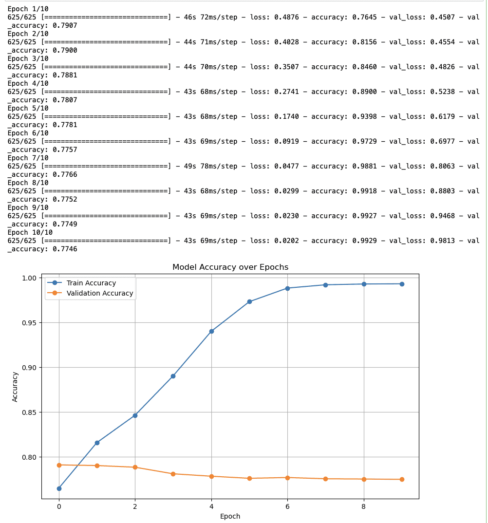
Here is the output.

Sentiment Analysis in Python: Going Beyond Bag of Words

Final Insights About Sentiment Analysis

Training Accuracy: The accuracy starts at nearly 80% and constantly increases to near 100% by the tenth epoch. So, it looks like the model is effectively learning.
Validation Accuracy: The validation accuracy again starts around 80% and continues steadily quickly, which could indicate that the model is not generalizing to unseen data.

At the beginning of this article, your interest was piqued. And let’s now explain the real story behind this.

The paper from Predicting Election Results from Twitter Using Machine Learning Algorithms,

published in “Recent Advances in Computer Science and Communications”, presents a machine learning-based method for predicting election results. Here you can read the whole.

In summary, they did sentiment analysis, and achieved 94.2 % accuracy, on the AP Assembly Election 2019. It looks like they really got close.

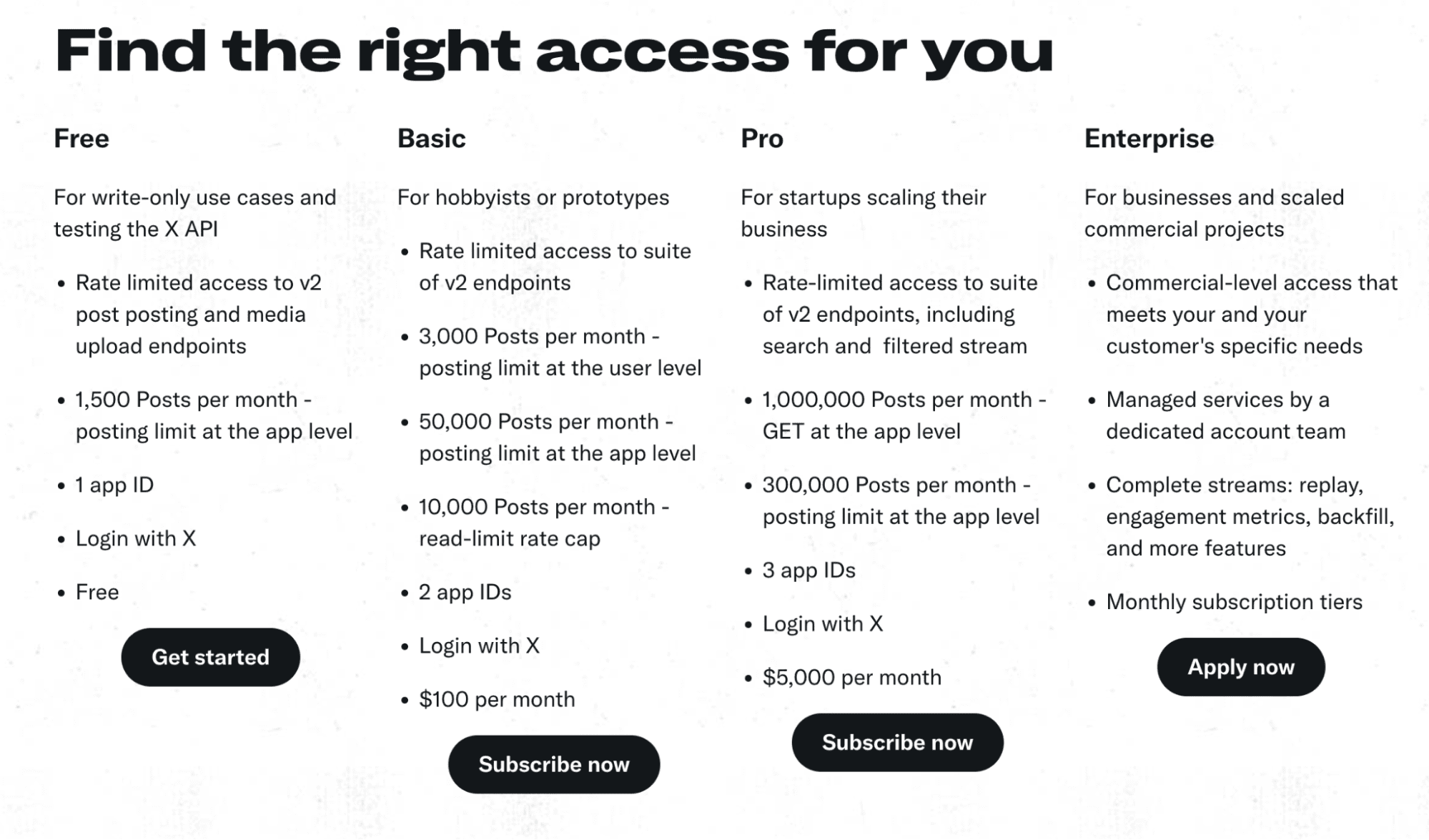
If you plan to do a portfolio project, research like this, or intend to go further from this case study, you can use Twitter API, or x API. Here are the plans: https://developer.twitter.com/en/products/twitter-api

Sentiment Analysis in Python: Going Beyond Bag of Words

You can do hashtag sentiment analysis on Twitter after major sports or political events. In 2024, there will be an election in a bunch of countries like the United States, where you can check the news.

The power of Data Science can really be seen in this example. This year, we will witness numerous elections worldwide, so if you aim to draw attention to your project, this might be a good idea. If you are a beginner searching for ways to learn data science, you can find many real-life projects, data science interview questions, and blog posts featuring data science projects like this on StrataScratch.

Nate Rosidi is a data scientist and in product strategy. He’s also an adjunct professor teaching analytics, and is the founder of StrataScratch, a platform helping data scientists prepare for their interviews with real interview questions from top companies. Connect with him on Twitter: StrataScratch or LinkedIn.