Simplify Amazon Redshift monitoring using the new unified SYS views | Amazon Web Services

Amazon Redshift is a fully managed, petabyte-scale data warehouse service in the cloud, providing up to five times better price-performance than any other cloud data warehouse, with performance innovation out of the box at no additional cost to you. Tens of thousands of customers use Amazon Redshift to process exabytes of data every day to power their analytics workloads.

In this post, we discuss Amazon Redshift SYS monitoring views and how they simplify the monitoring of your Amazon Redshift workloads and resource usage.

Overview of SYS monitoring views

SYS monitoring views are system views in Amazon Redshift that can be used to monitor query and workload resource usage for provisioned clusters as well as for serverless workgroups. They offer the following benefits:

• They’re categorized based on functional alignment, considering query state, performance metrics, and query types
• We have introduced new performance metrics like planning_time, lock_wait_time, remote_read_io, and local_read_io to aid in performance troubleshooting
• It improves the usability of monitoring views by logging the user-submitted query instead of the Redshift optimizer-rewritten query
• It provides more troubleshooting metrics using fewer views
• It enables unified Amazon Redshift monitoring by enabling you to use the same query across provisioned clusters or serverless workgroups

Let’s look at some of the features of SYS monitoring views and how they can be used for monitoring.

Unify various query-level monitoring metrics

The following table shows how you can unify various metrics and information for a query from multiple system tables & views into one SYS monitoring view.

For additional information on SYS to STL/SVL/STV mapping, refer to Migrating to SYS monitoring views.

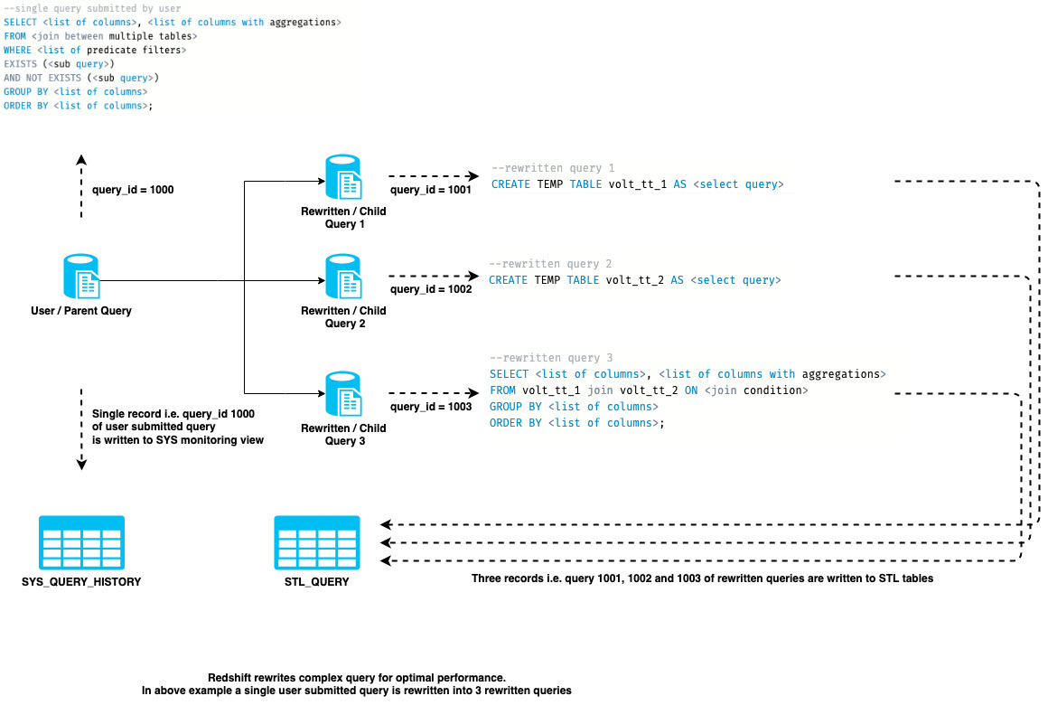
User query-level logging

To enhance query performance, the Redshift query engine can rewrite user-submitted queries. The user-submitted query identifier is different than the rewritten query identifier. We refer to the user-submitted query as the parent query and the rewritten query as the child query in this post.

The following diagram illustrates logging at the parent query level and child query level. The parent query identifier is 1000, and the child query identifiers are 1001, 1002, and 1003.

Query lifecycle timings

SYS_QUERY_HISTORY has an enhanced list of columns to provide granular time metrics relating to the different query lifecycle phases. Note all times are recorded in microseconds. The following table summarizes these metrics.

Solution overview

We discuss the following scenarios to help gain familiarity with the SYS monitoring views:

• Workload and query lifecycle monitoring
• Data ingestion monitoring
• External query monitoring
• Slow query performance troubleshooting

Prerequisites

You should have the following prerequisites to follow along with the examples in this post:

Additionally, download all the SQL queries that are referenced in this post as Redshift Query Editor v2 SQL notebooks.

Workload and query lifecycle monitoring

In this section, we discuss how to monitor the workload and query lifecycle.

Identify in-flight queries

SYS_QUERY_HISTORY provides a singular view to look at all the in-flight queries as well as historical runs. See the following example query:

SELECT *
FROM sys_query_history
WHERE status IN ('planning', 'queued', 'running', 'returning')
ORDER BY start_time;

We get the following output.

Identify top long-running queries

The following query helps retrieve the top 100 queries that are taking the longest to run. Analyzing (and, if feasible, optimizing) these queries can help improve overall performance. These metrics are accumulated statistics across all runs of the query. Note that all the time values are in microseconds.

--top long running query by elapsed_time
SELECT user_id , transaction_id , query_id , database_name , query_type , query_text::VARCHAR(100) , lock_wait_time , planning_time , compile_time , execution_time , elapsed_time
FROM sys_query_history
ORDER BY elapsed_time DESC
LIMIT 100;

We get the following output.

Gather daily counts of queries by query types, period, and status

The following query provides insight into the distribution of different types of queries across different days and helps evaluate and track any changes in the workload:

--daily breakdown of workload by query types and status
SELECT DATE_TRUNC('day', start_time) period_daily , query_type , status , COUNT(*)
FROM sys_query_history
GROUP BY period_daily , query_type , status
ORDER BY period_daily , query_type , status;

We get the following output.

Gather run details of an in-flight query

To determine the run-level details of a query that is in-flight, you can use the is_active = ‘t’ filter when querying the SYS_QUERY_DETAIL table. See the following example:

SELECT query_id , child_query_sequence , stream_id , segment_id , step_id , step_name , table_id , coalesce(table_name,'')|| coalesce(source,'') as table_name , start_time , end_time , duration , blocks_read , local_read_io , remote_read_io
FROM sys_query_detail
WHERE is_active = 't'
ORDER BY query_id , child_query_sequence , stream_id , segment_id , step_id;

To view the latest 100 COPY queries run, use the following code:

SELECT session_id , transaction_id , query_id , database_name , table_name , data_source , loaded_rows , loaded_bytes , duration / 1000.00 duration_ms
FROM sys_load_history
ORDER BY start_time DESC LIMIT 100;

We get the following output.

Gather transaction-level details for commits and undo

SYS_TRANSACTION_HISTORY provides transaction-level logging by providing insights into committed transactions with details like blocks committed, status, and isolation level (serializable or snapshot used). It also logs details about the rolled back or undo transactions.

The following screenshots illustrate fetching details about a transaction that was committed successfully.

The following screenshots illustrate fetching details about a transaction that was rolled back.

Stats and vacuum

The SYS_ANALYZE_HISTORY monitoring view provides details like the last timestamp of analyze queries, the duration for which a particular analyze query ran, the number of rows in the table, and the number of rows modified. The following example query provides a list of the latest analyze queries that ran for all the permanent tables:

SELECT TRIM(schema_name) schema_name , TRIM(table_name) table_name , table_id , status , COUNT(*) times_analyze_was_triggered , MAX(last_analyze_time) last_analyze_time , MAX(end_time) end_time , AVG(ROWS) "rows" , AVG(modified_rows) modified_rows
FROM sys_analyze_history
WHERE status != 'Skipped'
GROUP BY schema_name , table_name , table_id , status
ORDER BY schema_name , table_name , table_id , status , end_time;

We get the following output.

The SYS_VACUUM_HISTORY monitoring view provides a complete set of details on VACUUM in a single view. For example, see the following code:

SELECT user_id , transaction_id , query_id , TRIM(database_name) as database_name , TRIM(schema_name) as schema_name , TRIM(table_name) table_name , table_id , vacuum_type , is_automatic as is_auto , duration , rows_before_vacuum , size_before_vacuum , reclaimable_rows , reclaimed_rows , reclaimed_blocks , sortedrows_before_vacuum , sortedrows_after_vacuum
FROM sys_vacuum_history
WHERE status LIKE '%Finished%'
ORDER BY start_time;

We get the following output.

Data ingestion monitoring

In this section, we discuss how to monitor data ingestion.

Summary of ingestion

SYS_LOAD_HISTORY provides details into the statistics of COPY commands. Use this view for summarized insights into your ingestion workload. The following example query provides an hourly summary of ingestion broken down by tables in which data was ingested:

SELECT date_trunc('hour', start_time) period_hourly , database_name , table_name , status , file_format , SUM(loaded_rows) total_rows_ingested , SUM(loaded_bytes) total_bytes_ingested , SUM(source_file_count) num_of_files_to_process , SUM(file_count_scanned) num_of_files_processed , SUM(error_count) total_errors
FROM sys_load_history
GROUP BY period_hourly , database_name , table_name , status , file_format
ORDER BY table_name , period_hourly , status;

We get the following output.

File-level ingress logging

SYS_LOAD_DETAIL provides more granular insights into how ingestion is performed at the file level. For example, see the following query using sys_load_history:

SELECT *
FROM sys_load_history
WHERE table_name = 'catalog_sales'
ORDER BY start_time;

We get the following output.

The following example shows what detailed file-level monitoring looks like:

 SELECT user_id , query_id , TRIM(file_name) file_name , bytes_scanned , lines_scanned , splits_scanned , record_time , start_time , end_time
FROM sys_load_detail
WHERE query_id = 1824870
ORDER BY start_time;

Check for errors during ingress process

SYS_LOAD_ERROR_DETAIL enables you to track and troubleshoot errors that may have occurred during the ingestion process. This view logs details for the file that encountered the error during the ingestion process along with the line number at which the error occurred and column details within that line. See the following code:

select * from sys_load_error_detail order by start_time limit 100;

We get the following output.

External query monitoring

SYS_EXTERNAL_QUERY_DETAIL provides run details for external queries, which includes Amazon Redshift Spectrum and federated queries. This view logs details at the segment level and provides useful insights to troubleshoot and monitor performance of external queries in a single monitoring view. The following are a few useful metrics and data points this monitoring view provides:

• Number of external files scanned (scanned_files) and format of external files (file_format) such as Parquet, text file, and so on
• Data scanned in terms of rows (returned_rows) and bytes (returned_bytes)
• Usage of partitioning (total_partitions and qualified_partitions) by external queries and tables
• Granular insights into time taken in listing (s3list_time) and qualifying partitions (get_partition_time) for a given external object
• External file location (file_location) and external table name (table_name)
• Type of external source (source_type), such as Amazon Simple Storage Service (Amazon S3) for Redshift Spectrum, or federated
• Recursive scan for subdirectories (is_recursive) or access of nested column data type (is_nested)

For example, the following query shows the daily summary of the number of external queries run and data scanned:

SELECT DATE_TRUNC('hour', start_time) period_hourly , user_id , TRIM(source_type) source_type , COUNT (DISTINCT query_id) query_counts , SUM(returned_rows) returned_rows , ROUND(SUM(returned_bytes) / 1024^3,2) returned_gb
FROM sys_external_query_detail
GROUP BY period_hourly , user_id , source_type
ORDER BY period_hourly , user_id , source_type;

We get the following output.

Usage of partitions

You can verify whether the external queries scanning large sums of data and files are partitioned or not. When you use partitions, you can restrict the amount of data that your external query has to scan by pruning based on the partition key. See the following code:

SELECT file_location , CASE WHEN NVL(total_partitions,0) = 0 THEN 'No' ELSE 'Yes' END is_partitioned , SUM(scanned_files) total_scanned_files , COUNT(DISTINCT query_id) query_count
FROM sys_external_query_detail
GROUP BY file_location , is_partitioned
ORDER BY total_scanned_files DESC;

We get the following output.

For any errors encountered with external queries, look into SYS_EXTERNAL_QUERY_ERROR, which logs details at the granularity of file_location, column, and rowid within that file.

Slow query performance troubleshooting

Refer to the sysview_slow_query_performance_troubleshooting SQL notebook downloaded as part of the prerequisites for a step-by-step guide on how to perform query-level troubleshooting using SYS monitoring views and find answers to the following questions:

• Do the queries being compared have similar query text?
• Did the query use the result cache?
• Which parts of the query lifecycle (queuing, compilation, planning, lock wait) are contributing the most to query runtimes?
• Has the query plan changed?
• Is the query reading more data blocks?
• Is the query spilling to disk? If so, is it spilling to local or remote storage?
• Is the query highly skewed with respect to data (distribution) and time (runtime)?
• Do you see more rows processed in join steps or nested loops?
• Are there any alerts indicating staleness in statistics?
• When was the last vacuum and analyze performed for the tables involved in the query?

Clean up

If you created any Redshift provisioned clusters or Redshift Serverless workgroups as part of this post and no longer need them for your workloads, you can delete them to avoid incurring additional costs.

Conclusion

In this post, we explained how you can use the Redshift SYS monitoring views to monitor workloads of provisioned clusters and serverless workgroups. The SYS monitoring views provide simplified monitoring of the workloads, access to various query-level monitoring metrics from a unified view, and the ability to use the same SYS monitoring view query to run across both provisioned clusters and serverless workgroups. We also covered some key monitoring and troubleshooting scenarios using SYS monitoring views.

We encourage you to start using the new SYS monitoring views for your Redshift workloads. If you have any feedback or questions, please leave them in the comments.

About the authors

Urvish Shah is a Senior Database Engineer at Amazon Redshift. He has more than a decade of experience working on databases, data warehousing and in analytics space. Outside of work, he enjoys cooking, travelling and spending time with his daughter.

Ranjan Burman is a Analytics Specialist Solutions Architect at AWS. He specializes in Amazon Redshift and helps customers build scalable analytical solutions. He has more than 15 years of experience in different database and data warehousing technologies. He is passionate about automating and solving customer problems with the use of cloud solutions.

• SEO Powered Content & PR Distribution. Get Amplified Today.
• PlatoData.Network Vertical Generative Ai. Empower Yourself. Access Here.
• PlatoAiStream. Web3 Intelligence. Knowledge Amplified. Access Here.
• PlatoESG. Carbon, CleanTech, Energy, Environment, Solar, Waste Management. Access Here.
• PlatoHealth. Biotech and Clinical Trials Intelligence. Access Here.
• Source: https://aws.amazon.com/blogs/big-data/simplify-amazon-redshift-monitoring-using-the-new-unified-sys-views/