Undersampling Techniques Using Python – KDnuggets

With the evolving digital landscape, a wealth of data is being generated and captured from diverse sources. While immensely valuable, this vast universe of information often reflects the imbalanced distribution of real-world phenomena. The problem of imbalanced data is not merely a statistical challenge; it has far-reaching implications for the accuracy and reliability of the data-driven models.

Take, for example, the ever-growing and prevalent concern of fraud detection in the financial industry. As much as we want to avoid fraud due to its highly damaging nature, machines (and even humans) inevitably need to learn from the examples of fraudulent transactions (albeit rare) to distinguish them from the number of daily legitimate transactions. 

This imbalance in data distribution between fraudulent and non-fraudulent transactions poses significant challenges for the machine-learning models aimed at detecting such anomalous activities. Without appropriate handling of the data imbalance, these models risk becoming biased toward predicting transactions as legitimate, potentially overlooking the rare instances of fraud.

Healthcare is another field where machine learning models are leveraged to predict imbalanced outcomes, such as diseases like cancer or rare genetic disorders. Such outcomes occur far less frequently than their benign counterparts. Hence, the models trained on such imbalanced data are more susceptible to incorrect predictions and diagnoses. Such missed health alert defeats the purpose of the model in the first place, i.e., to detect early disease.

These are just a few instances highlighting the profound impact of data imbalance, i.e., where one class significantly outnumbers the other. Oversampling and Undersampling are two standard data preprocessing techniques to balance the dataset, of which we will focus on undersampling in this article. 

Let us discuss some popular methods for undersampling a given distribution.

Let’s start with an illustrative example to grasp the significance of under-sampling techniques better. The following visualization demonstrates the impact of the relative quantity of points per class, as executed by a Support Vector Machine with a linear kernel. The below code and plots are referred from the Kaggle notebook.

import matplotlib.pyplot as plt
from sklearn.svm import LinearSVC
import numpy as np
from collections import Counter
from sklearn.datasets import make_classification def create_dataset( n_samples=1000, weights=(0.01, 0.01, 0.98), n_classes=3, class_sep=0.8, n_clusters=1
): return make_classification( n_samples=n_samples, n_features=2, n_informative=2, n_redundant=0, n_repeated=0, n_classes=n_classes, n_clusters_per_class=n_clusters, weights=list(weights), class_sep=class_sep, random_state=0, ) def plot_decision_function(X, y, clf, ax): plot_step = 0.02 x_min, x_max = X[:, 0].min() - 1, X[:, 0].max() + 1 y_min, y_max = X[:, 1].min() - 1, X[:, 1].max() + 1 xx, yy = np.meshgrid( np.arange(x_min, x_max, plot_step), np.arange(y_min, y_max, plot_step) ) Z = clf.predict(np.c_[xx.ravel(), yy.ravel()]) Z = Z.reshape(xx.shape) ax.contourf(xx, yy, Z, alpha=0.4) ax.scatter(X[:, 0], X[:, 1], alpha=0.8, c=y, edgecolor="k") fig, ((ax1, ax2), (ax3, ax4)) = plt.subplots(2, 2, figsize=(15, 12)) ax_arr = (ax1, ax2, ax3, ax4)
weights_arr = ( (0.01, 0.01, 0.98), (0.01, 0.05, 0.94), (0.2, 0.1, 0.7), (0.33, 0.33, 0.33),
)
for ax, weights in zip(ax_arr, weights_arr): X, y = create_dataset(n_samples=1000, weights=weights) clf = LinearSVC().fit(X, y) plot_decision_function(X, y, clf, ax) ax.set_title("Linear SVC with y={}".format(Counter(y)))

The code above generates plots for four different distributions starting from a highly imbalanced dataset with one class dominating 97% of the instances. The second and third plots have 93% and 69% of the instances from a single class, respectively, while the last plot has a perfectly balanced distribution, i.e., all three classes contribute a third of the instances. Plots of the datasets from the most imbalanced to the least are displayed below. Upon fitting SVM over this data, the hyperplane in the first plot (highly imbalanced) is pushed to a side of the chart, mainly because the algorithm treats each instance equally, irrespective of the class, and tries to separate the classes with maximum margin. Hence, a majority yellow population near the center pushes the hyperplane to the corner, making the algorithm misclassify the minority classes.

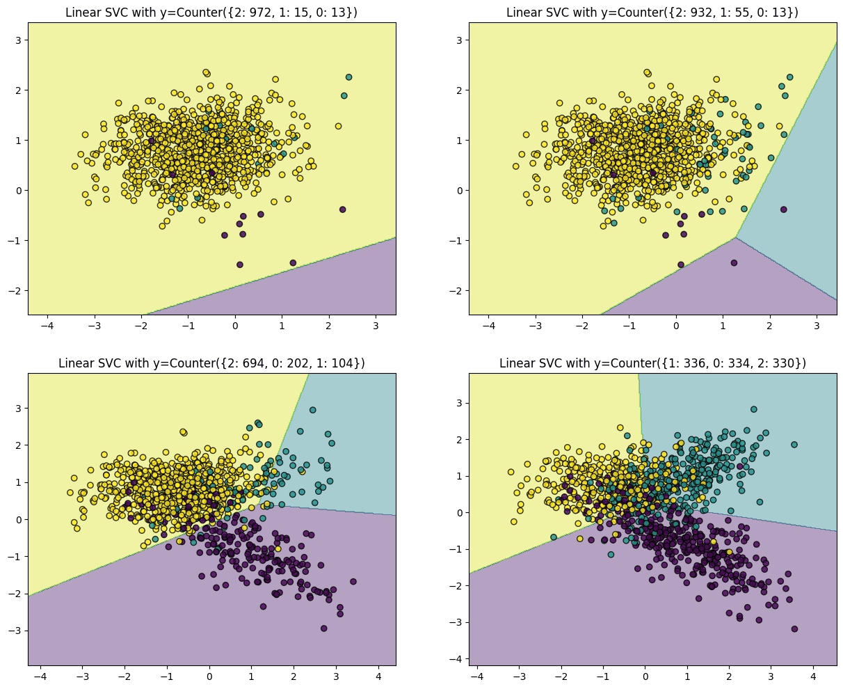
The algorithm successfully classifies all interest classes as we move towards a more balanced distribution.

In summary, when a dataset is dominated by one or a few classes, the resulting solution often results in a model with higher misclassifications. However, the classifier exhibits diminishing bias as the distribution of observations per class approaches an even split.

In this case, undersampling the yellow points presents the simplest solution to address model errors originating from the problem of rare classes. It’s worth noting that not all datasets encounter this issue, but for those that do, rectifying this imbalance forms a crucial preliminary step in modeling the data.

We’ll use the Imbalanced-Learn Python library (imbalanced-learn or imblearn). We can install it using pip:

pip install -U imbalanced-learn

Let us discuss and experiment with some of the most popular undersampling techniques. Suppose you have a binary classification dataset where class ‘0’ significantly outnumbers class ‘1’.

NearMiss Undersampling

NearMiss is an undersampling technique that reduces the number of majority samples closer to the minority class. This would facilitate clean classification by any algorithm using space separation or splitting the dimensional space between the two classes. There are three versions of NearMiss:

NearMiss-1: Majority class samples with a minimum average distance to the three closest minority class samples.

NearMiss-2: Majority class samples with a minimum average distance to three furthest minority class samples.

NearMiss-3: Majority class samples with minimum distance to each minority class sample.

Let’s demonstrate the NearMiss-1 undersampling algorithm through a code example:

# Import necessary libraries and modules
import numpy as np
import matplotlib.pyplot as plt
from collections import Counter
from sklearn.datasets import make_classification
from imblearn.under_sampling import NearMiss # Generate the dataset with different class weights
features, labels = make_classification( n_samples=1000, n_features=2, n_redundant=0, n_clusters_per_class=1, weights=[0.95, 0.05], flip_y=0, random_state=0,
) # Print the distribution of classes
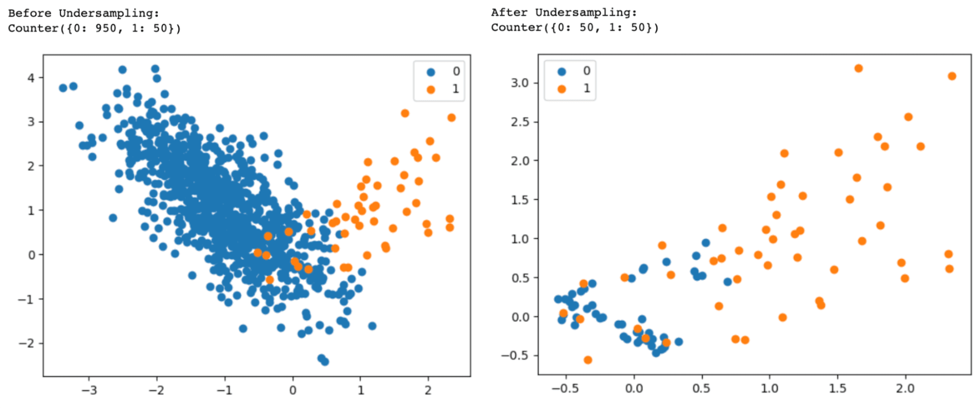
dist_classes = Counter(labels)
print("Before Undersampling:")
print(dist_classes) # Generate a scatter plot of instances, labeled by class
for class_label, _ in dist_classes.items(): instances = np.where(labels == class_label)[0] plt.scatter(features[instances, 0], features[instances, 1], label=str(class_label))
plt.legend()
plt.show() # Set up the undersampling method
undersampler = NearMiss(version=1, n_neighbors=3) # Apply the transformation to the dataset
features, labels = undersampler.fit_resample(features, labels) # Print the new distribution of classes
dist_classes = Counter(labels)
print("After Undersampling:")
print(dist_classes) # Generate a scatter plot of instances, labeled by class
for class_label, _ in dist_classes.items(): instances = np.where(labels == class_label)[0] plt.scatter(features[instances, 0], features[instances, 1], label=str(class_label))
plt.legend()
plt.show()

Change version=1 to version=2 or version=3 in the NearMiss() class to use the NearMiss-2 or NearMiss-3 undersampling algorithm.

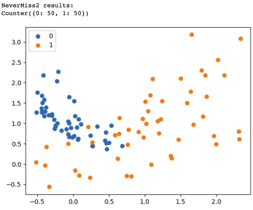
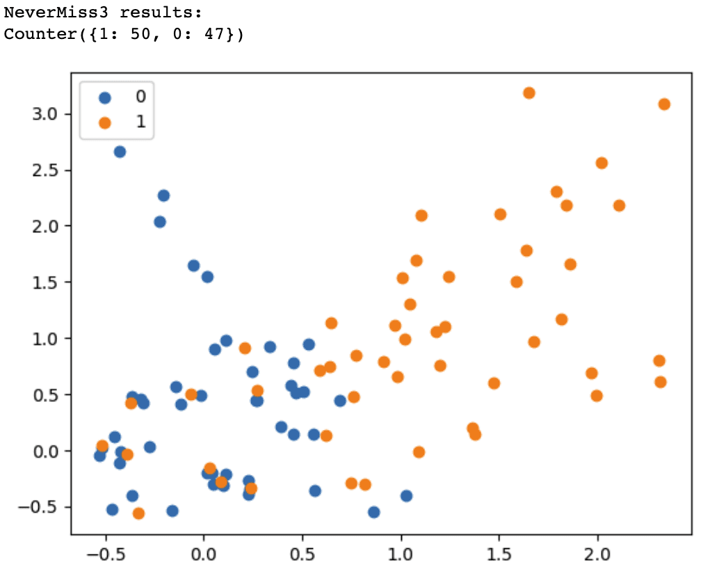
NearMiss-2 selects instances at the core of the overlap region between the two classes. With the NeverMiss-3 algorithm, we observe that every instance in the minority class, which overlaps with the majority class region, has up to three neighbors from the majority class. The attribute n_neighbors in the code sample above defines this.

This method starts by considering a subset of the majority class as noise. Then, it uses a 1-Nearest Neighbor algorithm to classify instances. If an instance from the majority class is misclassified, it’s included in the subset. The process continues until no more instances are included in the subset.

from imblearn.under_sampling import CondensedNearestNeighbour cnn = CondensedNearestNeighbour(random_state=42)
X_res, y_res = cnn.fit_resample(X, y)

Tomek Links are closely located pairs of opposite-class instances. Removing the instances of the majority class of each pair increases the space between the two classes, facilitating the classification process.

from imblearn.under_sampling import TomekLinks tl = TomekLinks()
X_res, y_res = tl.fit_resample(X, y) print('Original dataset shape:', Counter(y))
print('Resample dataset shape:', Counter(y_res))

With this, we have delved into the essential aspects of undersampling techniques in Python, covering three prominent methods: Near Miss Undersampling, Condensed Nearest Neighbour, and Tomek Links Undersampling. 

Undersampling is a crucial data processing step to address class imbalance problems in machine learning and also helps improve the model performance and fairness. Each of these techniques offers unique advantages and can be tailored to specific datasets and the goals of machine learning projects. 

This article provides a comprehensive understanding of the undersampling methods and their application in Python. I hope it enables you to make informed decisions on tackling class imbalance challenges in your machine-learning projects.
 
 

Vidhi Chugh is an AI strategist and a digital transformation leader working at the intersection of product, sciences, and engineering to build scalable machine learning systems. She is an award-winning innovation leader, an author, and an international speaker. She is on a mission to democratize machine learning and break the jargon for everyone to be a part of this transformation.

• SEO Powered Content & PR Distribution. Get Amplified Today.
• PlatoData.Network Vertical Generative Ai. Empower Yourself. Access Here.
• PlatoAiStream. Web3 Intelligence. Knowledge Amplified. Access Here.
• PlatoESG. Carbon, CleanTech, Energy, Environment, Solar, Waste Management. Access Here.
• PlatoHealth. Biotech and Clinical Trials Intelligence. Access Here.
• Source: https://www.kdnuggets.com/undersampling-techniques-using-python?utm_source=rss&utm_medium=rss&utm_campaign=undersampling-techniques-using-python