Unleashing the Power of Few Shot Learning

Introduction

Welcome to the realm of few-shot learning, where machines defy the data odds and learn to conquer tasks with just a sprinkle of labeled examples. In this guide, we’ll embark on a thrilling journey into the heart of few-shot learning. We will explore how these clever algorithms achieve greatness with minimal data, opening doors to new possibilities in artificial intelligence.

Learning Objectives

Before we dive into the technical details, let’s outline the learning objectives of this guide:

• Understanding the concept, how it differs from traditional machine learning, and the importance of this approach in data-scarce scenarios
• Explore various methodologies and algorithms used in few-shot learning, such as metric-based methods, model-based approaches, and their underlying principles.
• How to apply few-shot learning techniques in different scenarios? Understand best practices for effectively training and evaluating few-shot learning models.
• Discover real-world applications of Few-Shot Learning.
• Understanding the Advantages and Limitations of Few-Shot Learning

Now, let’s delve into each section of the guide and understand how to accomplish these objectives.

This article was published as a part of the Data Science Blogathon.

What is Few Shot Learning?

Few-shot learning is a subfield of machine learning that addresses the challenge of training models to recognize and generalize from a limited number of labeled examples per class or task. Few-shot learning is a subfield of machine learning that challenges the traditional notion of data-hungry models. Instead of relying on massive datasets, few-shot learning enables algorithms to learn from only a handful of labeled samples. This ability to generalize from scarce data opens up remarkable possibilities in scenarios where acquiring extensive labeled datasets is impractical or expensive.

Picture a model that can quickly grasp new concepts, recognize objects, understand complex languages, or make accurate predictions even with limited training examples. Few-shot learning empowers machines to do just that, transforming how we approach various challenges across diverse domains. The primary objective of few-shot learning is to develop algorithms and techniques that can learn from scarce data and generalize well to new, unseen instances. It often involves leveraging prior knowledge or leveraging information from related tasks to generalize to new tasks efficiently.

Key Differences From Traditional Machine Learning

Traditional machine learning models typically require much-labeled data for training. The performance of these models tends to improve as the volume of data increases. In traditional machine learning, data scarcity can be a significant challenge, particularly in specialized domains or when acquiring labeled data is costly and time-consuming. Few-shot learning models learn effectively with only a few examples per class or task. These models can make accurate predictions even when trained on just a few or a single labeled example per class. It addresses the data scarcity problem by training models to learn effectively with minimal labeled data. Adapt quickly to new classes or tasks with just a few updates or adjustments.

Few Shot Learning Terminologies

In the field of few-shot learning, several terminologies and concepts describe different aspects of the learning process and algorithms. Some key terminologies commonly in few-shot learning:

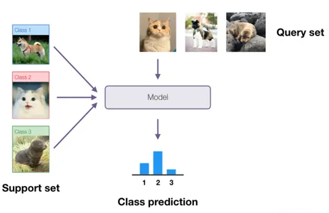
• Support Set: The support set is a subset of the dataset in few-shot learning tasks. It contains a limited number of labeled examples (images, text samples, etc.) for each class in the dataset. The purpose of the support set is to provide the model with relevant information and examples to learn and generalize about the classes during the meta-training phase.
• Query Set: The query set is another subset of the dataset in few-shot learning tasks. It consists of unlabeled examples (images, text samples, etc.) that must be classified into one of the classes present in the support set. After training on the support set, evaluate the model’s performance on how accurately it can classify the query set examples.
• N-Way K-Shot: In few-shot learning, “n-way k-shot” is a standard notation to describe the number of classes (n) and the number of support examples per class (k) in each few-shot learning episode or task. For example, “5-way 1-shot” means that each episode contains five classes, and the model is provided with only one support example per class. Similarly, “5-way 5-shot” means five classes are in each episode, and the model is provided with five support examples per class.

Few Shot Learning Techniques

Metric-Based Approaches

• Siamese Networks: Siamese networks learn to compute embeddings (representations) for input samples and then use distance metrics to compare the embeddings for similarity-based classification. It compares and measures the similarity between two inputs and is particularly useful when examples exist for each class. In the context of few-shot learning, utilize the Siamese networks to learn a similarity metric between support set examples and query set examples. The support set consists of labeled examples (e.g., one or a few examples per class), while the query set contains unlabeled examples that need to be classified into one of the classes present in the support set.
• Prototypical Networks: It is a popular and effective approach in few-shot learning tasks. Prototypical networks use the idea of “prototypes” for each class, which are the average embeddings of the few-shot examples. The query sample compares the prototypes during inference to determine their class. The key idea is to represent each class by computing a prototype vector as the mean of the feature embeddings of its support set examples. During inference, a query example is classified based on its proximity to the prototypes of different classes. They are computationally efficient and do not require complex meta-learning strategies, making them a popular choice for practical implementations in various domains, including computer vision and natural language processing.

Model-Based Approaches

• Memory-Augmented Networks: Memory-augmented networks (MANNs) employ external memory to store information from few-shot examples. They use attention mechanisms to retrieve relevant information during classification. MANNs aim to overcome the limitations of standard neural networks, which often struggle with tasks requiring large context information or long-range dependencies. The key idea behind MANNs is to equip the model with a memory module that can read and write information, allowing it to store relevant information during training and use it during inference. This external memory is an additional resource that the model can access and update to facilitate reasoning and decision-making.
• Meta-Learning (Learning to Learn): Meta-learning aims to improve few-shot learning by training models to quickly adapt to new tasks based on a meta-training phase with various tasks. The core idea behind meta-learning is to enable models to extract knowledge from previous experiences (meta-training) and use that knowledge to adapt quickly to new, unseen tasks (meta-testing). Meta-learning addresses these challenges by introducing the concept of “meta-knowledge” or “prior knowledge” that guides the model’s learning process.
• Gradient-Based Meta-Learning (e.g., MAML): Gradient-based meta-learning modifies model parameters to facilitate faster adaptation to new tasks during meta-testing. The primary goal of MAML is to enable models to quickly adapt to new tasks with only a few examples, a central theme in few-shot learning and meta-learning scenarios.

Applications of Few Shot Learning

Few-shot learning has numerous practical applications across various domains. Here are some notable applications of few-shot learning:

1. Image Classification and Object Recognition: In image classification tasks, models can quickly recognize and classify objects with limited labeled examples. It is especially useful for recognizing rare or novel objects not present in the training dataset.
2. Natural Language Processing: In NLP, few-shot learning enables models to perform tasks like sentiment analysis, text classification, and named entity recognition with minimal labeled data. It is beneficial in scenarios where labeled text data is scarce or expensive to obtain.
3. Medical Diagnosis and Healthcare: Few-shot learning holds promise in medical imaging analysis and diagnosis. It can aid in identifying rare diseases, detecting anomalies, and predicting patient outcomes with limited medical data.
4. Recommendation Systems: Suggest personalized content or products to users based on a small number of user interactions or preferences.
5. Personalized Marketing and Advertisement: Help businesses target specific customer segments with personalized marketing campaigns based on limited customer data.

Advantages of Few Shot Learning

1. Data Efficiency: Few-shot learning requires only a small number of labeled examples per class, making it highly data-efficient. This is particularly advantageous when acquiring large labeled datasets is expensive or impractical.
2. Generalization to New Tasks: Few-shot learning models excel at quickly adapting to new tasks or classes with minimal labeled examples. This flexibility allows them to handle unseen data efficiently, making them suitable for dynamic and evolving environments.
3. Rapid Model Training: With fewer examples to process, train the models quickly compared to traditional ML models that require extensive labeled data.
4. Handling Data Scarcity: directly addresses the issue of data scarcity, enabling models to perform well even when training data is scarce or unavailable for specific classes or tasks.
5. Transfer Learning: Few-shot learning models inherently possess transfer learning capabilities. The knowledge from few-shot classes transfers to improve performance on related tasks or domains.
6. Personalization and Customization: Facilitate personalized and customized solutions, as models can quickly adapt to individual user preferences or specific requirements.
7. Reduced Annotation Efforts: Reduces the burden of manual data annotation, requires fewer labeled examples for training, saving time and resources.

Limitations

1. Limited Class Discrimination: The setting may not provide enough examples to capture fine-grained class differences, leading to reduced discriminative power for closely related classes.
2. Dependency on Few-Shot Examples: The models heavily rely on the quality and representativeness of the few-shot examples provided during training.
3. Task Complexity: Few-shot learning may struggle with highly complex tasks that demand a deeper understanding of intricate patterns in the data. It may require a more extensive set of labeled examples or a different learning paradigm.
4. Vulnerable to Noise: More sensitive to noisy or erroneous labeled examples, as fewer data points are needed for learning.
5. Data Distribution Shift: Models may struggle when the test data distribution significantly deviates from the few-shot training data distribution.
6. Model Design Complexity: Designing effective few-shot learning models often involves more intricate architectures and training methodologies, which can be challenging and computationally expensive.
7. Difficulty with Outliers: The models may struggle with outliers or rare instances that are significantly different from the few-shot examples seen during training

Practical Implementation of Few-Shot Learning

Let’s take an example of a few-shot image classification task.

We will be classifying images of different objects into their respective classes. The images belong to three classes: “cat”, “dog”, and “tulip.” The goal of the classification task is to predict the class label (i.e., “cat”, “dog”, or “tulip”) for a given query image based on its similarity to the prototypes of the classes in the support set. The first step is data preparation. Obtain and preprocess the few-shot learning dataset, dividing it into support (labeled) and query (unlabeled) sets for each task. Ensure the dataset represents the real-world scenarios the model will encounter during deployment. Here we collect a diverse dataset of images containing various animal and plant species, labeled with their respective classes. For each task, randomly select a few examples (e.g., 1 to 5 images) as the support set.

These support images will be used to “teach” the model about the specific class. The images for the same class form the query set and evaluate the model’s ability to classify unseen instances. Create multiple few-shot tasks by randomly selecting different classes and creating support and query sets for each task. Apply data augmentation techniques to augment the support set images, such as random rotations, flips, or brightness adjustments. Data augmentation helps increase the support set’s adequate size and improve the model’s robustness. Organize the data into pairs or mini-batches, each consisting of the support set and the corresponding query set.

Examples

For example, a few-shot task might look like this:

1:

• Support Set: [cat_1.jpg, cat_2.jpg, cat_3.jpg]
• Query Set: [cat_4.jpg, cat_5.jpg, cat_6.jpg, cat_7.jpg]

2:

• Support Set: [dog_1.jpg, dog_2.jpg]
• Query Set: [dog_3.jpg, dog_4.jpg, dog_5.jpg, dog_6.jpg]

3:

• Support Set: [tulip_1.jpg, tulip_2.jpg]
• Query Set: [tulip_3.jpg, tulip_4.jpg, tulip_5.jpg, tulip_6.jpg]

And so on…

import numpy as np
import random # Sample dataset of images and their corresponding class labels
dataset = [ {"image": "cat_1.jpg", "label": "cat"}, {"image": "cat_2.jpg", "label": "cat"}, {"image": "cat_3.jpg", "label": "cat"}, {"image": "cat_4.jpg", "label": "cat"}, {"image": "dog_1.jpg", "label": "dog"}, {"image": "dog_2.jpg", "label": "dog"}, {"image": "dog_3.jpg", "label": "dog"}, {"image": "dog_4.jpg", "label": "dog"}, {"image": "tulip_1.jpg", "label": "tulip"}, {"image": "tulip_2.jpg", "label": "tulip"}, {"image": "tulip_3.jpg", "label": "tulip"}, {"image": "tulip_4.jpg", "label": "tulip"},
] # Shuffle the dataset
random.shuffle(dataset) # Split dataset into support and query sets for a few-shot task
num_support_examples = 3
num_query_examples = 4 few_shot_task = dataset[:num_support_examples + num_query_examples] # Prepare support set and query set
support_set = few_shot_task[:num_support_examples]
query_set = few_shot_task[num_support_examples:]#import csv

A simple function, load_image, is defined to simulate image loading, and another function, get_embedding, is defined to simulate image feature extraction (embedding). In this implementation, the load_image function uses PyTorch’s transforms to preprocess the image and convert it to a tensor. The function loads a pre-trained ResNet-18 model from the PyTorch model hub, performs a forward pass on the image, and extracts features from one of the intermediate convolutional layers. Flatten and convert the features to a NumPy array, which will calculate the embeddings and distances in the few-shot learning example.

def load_image(image_path): image = Image.open(image_path).convert("RGB") transform = transforms.Compose([ transforms.Resize((224, 224)), transforms.ToTensor(), transforms.Normalize(mean=[0.485, 0.456, 0.406], std=[0.229, 0.224, 0.225]) ]) return transform(image) # Generate feature embeddings for images using a pre-trained CNN (e.g., ResNet-18)
def get_embedding(image): model = torch.hub.load('pytorch/vision', 'resnet18', pretrained=True) model.eval() with torch.no_grad(): image = image.unsqueeze(0) # Add batch dimension to the image tensor features = model(image) # Forward pass through the model to get features # Return the feature embedding (flatten the tensor) return features.squeeze().numpy()#import csv

Few-shot Learning Technique

Select a suitable few-shot learning technique based on your specific task requirements and available resources.

# Create prototypes for each class in the support set
class_prototypes = {}
for example in support_set: image = load_image(example["image"]) embedding = get_embedding(image) if example["label"] not in class_prototypes: class_prototypes[example["label"]] = [] class_prototypes[example["label"]].append(embedding) for label, embeddings in class_prototypes.items(): class_prototypes[label] = np.mean(embeddings, axis=0) for query_example in query_set: image = load_image(query_example["image"]) embedding = get_embedding(image) distances = {label: np.linalg.norm(embedding - prototype) for label, prototype in class_prototypes.items()} predicted_label = min(distances, key=distances.get) print(f"Query Image: {query_example['image']}, Predicted Label: {predicted_label}")

This is a basic few-shot learning setup for image classification using Prototypical Networks. The code creates prototypes for each class in the support set. Prototypes are computed as the mean of the embeddings of support examples in the same class. Prototypes represent the central point of the feature space for each class. For each query example in the query set, the code calculates the distance between the query example’s embedding and the prototypes of each class in the support set. The query example is assigned to the class with the nearest prototype based on the calculated distances. Finally, the code prints the query image’s filename and the predicted class label based on the few-shot learning process.

# Loss function (Euclidean distance)
def euclidean_distance(a, b): return np.linalg.norm(a - b) # Calculate the loss (negative log-likelihood) for the predicted class
query_label = query_example["label"]
loss = -np.log(np.exp(-euclidean_distance(query_set_prototype, class_prototypes[query_label])) / np.sum(np.exp(-euclidean_distance(query_set_prototype, prototype)) for prototype in class_prototypes.values())) print(f"Loss for the Query Example: {loss}")#import csv

After computing the distances between the query set prototype and each class prototype, we calculate the loss for the predicted class using the negative log-likelihood (cross-entropy loss). The loss penalizes the model if the distance between the query set prototype and the correct class prototype is large, encouraging the model to minimize this distance and correctly classify the query example.

This was the simple implementation. Following is the complete implementation of the few-shot learning example with Prototypical Networks, including the training process:

import numpy as np
import random
import torch
import torch.nn as nn
import torchvision.transforms as transforms
from torch.optim import Adam
from PIL import Image # Sample dataset of images and their corresponding class labels
# ... (same as in the previous examples) # Shuffle the dataset
random.shuffle(dataset) # Split dataset into support and query sets for a few-shot task
num_support_examples = 3
num_query_examples = 4 few_shot_task = dataset[:num_support_examples + num_query_examples] # Prepare support set and query set
support_set = few_shot_task[:num_support_examples]
query_set = few_shot_task[num_support_examples:] # Helper function to load an image and transform it to a tensor
def load_image(image_path): image = Image.open(image_path).convert("RGB") transform = transforms.Compose([ transforms.Resize((224, 224)), transforms.ToTensor(), transforms.Normalize(mean=[0.485, 0.456, 0.406], std=[0.229, 0.224, 0.225]) ]) return transform(image) # Generate feature embeddings for images using a pre-trained CNN (e.g., ResNet-18)
def get_embedding(image): model = torch.hub.load('pytorch/vision', 'resnet18', pretrained=True) model.eval() # Extract features from the image using the model's convolutional layers with torch.no_grad(): image = image.unsqueeze(0) # Add batch dimension to the image tensor features = model(image) # Forward pass through the model to get features # Return the feature embedding (flatten the tensor) return features.squeeze() # Prototypical Networks Model
class PrototypicalNet(nn.Module): def __init__(self, input_size, output_size): super(PrototypicalNet, self).__init__() self.input_size = input_size self.output_size = output_size self.fc = nn.Linear(input_size, output_size) def forward(self, x): return self.fc(x) # Training
num_classes = len(set([example['label'] for example in support_set]))
input_size = 512 # Size of the feature embeddings (output of the CNN)
output_size = num_classes # Create Prototypical Networks model
model = PrototypicalNet(input_size, output_size) # Loss function (Cross-Entropy)
criterion = nn.CrossEntropyLoss() # Optimizer (Adam)
optimizer = Adam(model.parameters(), lr=0.001) # Training loop
num_epochs = 10 for epoch in range(num_epochs): model.train() # Set the model to training mode for example in support_set: image = load_image(example["image"]) embedding = get_embedding(image) # Convert the class label to a tensor label = torch.tensor([example["label"]]) # Forward pass outputs = model(embedding) # Compute the loss loss = criterion(outputs, label) # Backward and optimize optimizer.zero_grad() loss.backward() optimizer.step() print(f"Epoch [{epoch+1}/{num_epochs}], Loss: {loss.item():.4f}") # Inference (using the query set)
model.eval() # Set the model to evaluation mode query_set_embeddings = [get_embedding(load_image(example["image"])) for example in query_set] # Calculate the prototype of the query set
query_set_prototype = torch.mean(torch.stack(query_set_embeddings), dim=0) # Classify each query example
predictions = model(query_set_prototype) # Get the predicted labels
_, predicted_labels = torch.max(predictions, 0) # Get the predicted label for the query example
predicted_label = predicted_labels.item() # Print the predicted label for the query example
print(f"Query Image: {query_set[0]['image']}, Predicted Label: {predicted_label}")

In this complete implementation, we define a simple Prototypical Networks model and perform training using a Cross-Entropy loss and Adam optimizer. After training, we use the trained model to classify the query example based on the Prototypical Networks approach.

Future Directions and Potential Applications

This field has shown remarkable progress but is still evolving with many promising future directions and potential applications. Here are some of the key areas of interest for the future:

1. Continued Advances in Meta-Learning: are likely to see further developments. Improvements in optimization algorithms, architectural designs, and meta-learning strategies may lead to more efficient and effective few-shot learning models. Research on addressing challenges in catastrophic forgetting and the scalability of meta-learning methods is ongoing.
2. Incorporating Domain Knowledge: Integrating domain knowledge into few-shot learning algorithms can enhance their ability to generalize and transfer knowledge across different tasks and domains. Combining few-shot learning with symbolic reasoning or structured knowledge representation could be promising.
3. Exploring Hierarchical Few-Shot Learning: Extending the hierarchical settings, where tasks and classes are organized hierarchically, can enable models to exploit hierarchical relationships between classes and tasks, leading to better generalization.
4. Few-Shot Reinforcement Learning: Integrating them with reinforcement learning can enable agents to learn new tasks with limited experience. This area is particularly relevant for robotic control and autonomous systems.
5. Adapting to Real-World Applications: The application and real-world scenarios, such as medical diagnosis, drug discovery, personalized recommendation systems, and adaptive tutoring, hold significant promise. Future research may focus on developing specialized few-shot learning techniques tailored to specific domains.

Conclusion

It is a captivating subfield of AI and machine learning addressing the challenge of training models with minimal data. Throughout this blog, we explored its definition, differences from traditional ML, Prototypical Networks, and real-world applications in medical diagnosis and personalized recommendations. Exciting research directions include meta-learning, graph neural networks, and attention mechanisms, propelling AI to adapt quickly and make accurate predictions.

By democratizing AI and enabling adaptability with limited data, it opens doors for wider AI adoption. This journey towards unlocking untapped potential will lead to a future where machines and humans coexist harmoniously, shaping a more intelligent and beneficial AI landscape.

Key Takeaways

• Few-shot learning is an intriguing subfield of artificial intelligence and machine learning that addresses the challenge of training models with limited labeled examples.
• Prototypical Networks are powerful techniques used, enabling models to adapt and efficiently predict with limited labeled data.
• It has real-world applications in medical diagnosis and personalized recommendations, showcasing its versatility and practicality. It can potentially democratize AI by reducing the dependency on vast amounts of labeled data.

Frequently Asked Questions

The media shown in this article is not owned by Analytics Vidhya and is used at the Author’s discretion.

Related

• SEO Powered Content & PR Distribution. Get Amplified Today.
• PlatoData.Network Vertical Generative Ai. Empower Yourself. Access Here.
• PlatoAiStream. Web3 Intelligence. Knowledge Amplified. Access Here.
• PlatoESG. Automotive / EVs, Carbon, CleanTech, Energy, Environment, Solar, Waste Management. Access Here.
• BlockOffsets. Modernizing Environmental Offset Ownership. Access Here.
• Source: https://www.analyticsvidhya.com/blog/2023/07/few-shot-learning/