An all-in-one nanoprinting approach for the synthesis of a nanofilm library for unclonable anti-counterfeiting applications – Nature Nanotechnology

Solvent-free synthesis process

Film preparation

Typically, 1 g d-(+)-glucosamine hydrochloride (99%, Sigma) was dissolved in 3 ml H₂O. A clean glass slide was covered by a scotch tape (3M company) frame with a defined 1.5 cm × 1.5 cm area (Supplementary Fig. 1). We deposited 300 µl of the solution on the surface of the glass and dried it in an oven at 50 °C for around 30 min. Afterwards, the tape was removed and the film was placed in an air oven for thermal annealing.

Characterization

The annealed films were removed from the surface and dissolved with 2 ml H₂O in Eppendorf tubes. After centrifuging at 9,391g (10,000 r.p.m.) for 10 min, the supernatant was filtered through a 0.45 µm hydrophilic filter (CHROMAFIL Xtra, 13 mm). The obtained solution was used for the following characterizations. Ultraviolet–visible spectra were recorded with a UV-1900 spectrometer (Shimadzu). Fluorescence spectra of CDs were measured using a microplate reader (SpectraMax M5, Molecular Devices). Mass spectra were recorded using an HPLC-System Series 1100 coupled with ESI-single quadrupole from Agilent. NMR spectra were obtained on an AscendTM 400 spectrometer (400 MHz, Bruker) at 298 K, and are reported in ppm relative to the residual solvent peaks. For ¹H and ¹³C spectra, the films were directly dissolved in 600 µl D₂O (Sigma) before centrifugation and filtration. The TEM study was performed using a double Cs corrected JEOL JEM-ARM200F (scanning) transmission electron microscope operated at 80 kV and equipped with a cold-field emission gun. Annular dark-field scanning transmission electron microscopy images were collected at a probe convergence semi-angle of 25 mrad. Atomic force microscopy measurements were recorded with a JPK Bruker NanoWizard4 instrument in a.c. (tapping) mode.

Colour coordinate calculation

The colour coordinates of fluorescence were presented in CIE 1931 colour space according to the standard of the International Commission on Illumination. In a typical test, the emission intensities (Em) of material were collected every 5 nm in the wavelength range between (excitation wavelength + 20) nm and 700 nm to avoid the influence of the excitation resource. Multiple emission spectra were obtained under different excitation wavelengths in the range between 300 and 600 nm (20 nm steps), finally producing a 2D fluorescence spectrum for the studied material. Before calculation, all Em were normalized by the highest Em in the 2D fluorescence spectrum and only major emission spectra were taken into consideration (normalized Em_max > 0.5).

Temperature diffusion simulation

The temperature diffusion during the laser irradiation process was simulated by ANSYS with a steady-state thermal analysis system. The geometry model was constructed using 3dsMax as a file in SAT format. Standard engineering data were used, including the thermal conductivity of industrial glass, haematite and glucose. The model was automatically meshed by the MultiZone method with no suppression. The initial temperature of the irradiated laser spot was set to 25 °C (environment temperature), the final point was set to 1,000 °C. Thermal convection of all faces of the model were taken into consideration. The simulation lasted for 1 s.

nanoFlash approach

Preparation of donor slides

Absorber layer

The haematite films were generated based on our previous work⁴⁷. Briefly, two solutions need to be prepared and mixed: 125 mg of PVA (average M_r ≈ 9,000–10,000, Sigma) and 125 mg of Fe(NO₃)₃·9H₂O (98%, Acros) in 250 µl of double-distilled H₂O; 250 mg of PEG (average M_r ≈ 20,000, Sigma) and 250 mg of Fe(NO₃)₃·9H₂O in 250 µl of methanol. Then, the solution was spin-coated onto a clean glass slide at 70 r.p.s. and the slide was annealed in an air oven at 500 °C for 3 h. After cooling down, the final haematite layer was obtained. For the CuO absorber layer, we dissolved 0.175 g Cu(NO₃)₂·xH₂O (99%, Acros) and 0.175 g PVA (average M_r ≈ 9,000–10,000, Sigma) in 0.5 ml of H₂O and spin-coated the solution onto a glass slide at 70 r.p.s. Then, the slide was annealed at 500 °C for 3 h in an air oven. After cooling down, the final CuO layer was obtained as a black film.

Material layer

First, 25 mg (or 50, 100, 150 mg, depending on the specific recipes) of d-(+)-glucose (Merck) was dissolved in 500 µl of H₂O. We spin-coated the solution onto the absorber layer at 70 r.p.s. to obtain a homogeneous material layer. By replacing d-glucose with d-(+)-glucosamine hydrochloride (99%, Sigma), d-galactose (Carbosynth) or N-acetylglucosamine (99%, Sigma), material layers with other precursors were obtained.

Printing process

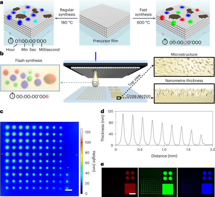
After cleaning the back side of the donor slide, we placed it on top of a clean glass which served as the acceptor slide. During the printing process, we use a 200 mW TOPTICA iBeam smart 488-S laser (488 nm, TOPTICA Photonics), which is passed through a 1:10 beam expander and a Racoon 11 laser scan head (ARGES) equipped with an f-Theta lens. The generated patterns were generally characterized by fluorescent images with a high-resolution fluorescence scanner (Innopsys, Innoscan 1100AL) at a pixel resolution of 5 µm and a scanning speed of 25 lines per second. The red channel was excited at 635 nm with an emission filter of 680/42; the green channel was excited at 532 nm with an emission filter of 605/15; the blue channel was excited at 488 nm with an emission filter of 520/5. Detection was performed with a gain factor of 5 and low laser power. The thickness information was gained by vertical scanning interferometry with a smartWLI compact (Gesellschaft für Bild- und Signalverarbeitung). For morphology analysis, scanning electron microscopy was carried out using a Zeiss LEO 1550 microscope equipped with a field emission gun and with an Oxford Instruments X-MAX SDD X-ray energy-dispersive detector (detection area, 80 mm²); images were recorded at 3 kV.

Library preparation

The precursor type and concentration, absorber material and thickness, and additives are the factors that could be tuned during the preparation of donor slides. Different laser foci were achieved by adjusting the distance of the sample stage from the scan head. In the focus plane, the laser spot was measured with a 1/e² diameter of 18 µm as reported previously⁴⁸. Other planes, which result in larger laser spots, are defined as the low focus area. The scanning speed, laser power and printing mode (optimized line scanning versus bitmap scanning) are controlled by the laser scanning system.

Machine learning

Extraction of the dataset

The fluorescent films generated in the library were used to obtain the dataset. The fluorescence intensity from three channels was read from CSV files exported by the high-resolution scanner and the mean value of the intensity was recorded in the dataset. Data cleaning was conducted to fix or remove incorrect, duplicate or incomplete data. After obtaining a dataset suitable for training, the dataset was then shuffled and divided into the training set and test set at a ratio of 4:1. We used one-shot encoding for categoric features, which expanded the value of discrete features to Euclidean space and solved the problem that the model could not directly deal with categoric features.

Machine learning models

We introduced different regression models to predict the fluorescence intensity. Scikit-Learn was used to obtain the algorithms of support vector machine regression (SVR), multilayer perceptron (MLP), k-nearest neighbours regression (KNN), polynomial regression (PR), decision tree regression (DT) and random forest regression (RF). The construction of XGB was performed using another independent library. Before the SVR, PR, KNN and MLP training, we normalized the features so that all of the variables are in the same range. Normalization also accelerated the gradient descent to find the optimal solution. For tree-based models (DT, RF and XGB), this step was not necessary. The repeated k-fold cross-validation procedure with 5 folds and 10 repeats was used to evaluate each algorithm. Importantly, all algorithms were configured with the same random seed to ensure that the same splits to the training data are performed, so each algorithm was precisely evaluated in the same way. The optimal hyperparameters for models were found by grid-search.

LoFTR algorithm

The LoFTR algorithm is a framework for image feature matching. Instead of performing image feature detection, description and matching one by one sequentially, it first establishes a pixel-wise dense match and refines the matches later. In contrast to traditional methods that utilize a cost volume to search corresponding matches, the framework applies self- and cross-attention layers from its Transformer model to obtain feature descriptors on both images. The global receptive field provided by Transformer enables the LoFTR algorithm to produce dense matches, even in low-texture areas, where traditional feature detectors usually struggle to produce repeatable interest points. Furthermore, the framework model is pretrained on indoor and outdoor datasets to detect the kind of image being analysed, with features such as self-attention. Hence, LoFTR outperforms other state-of-the-art methods. The LoFTR module uses self- and cross-attention layers in Transformers to transform the local features to be context- and position-dependent, which is crucial for LoFTR to obtain high-quality matches on indistinctive regions with low-texture or repetitive patterns. For image pair (I^A, I^B), their similarity is defined by the number of matched features:

where N_matches(I^A, I^B) is the number of matched features and N_features is the number of extracted features. The LoFTR algorithm extracts 4,800 features in total; however, for the border area, a mask has been applied for practical analysis. Therefore, the maximum number of possible extracted features is 4,256. The resulting colourmap shows the matching probability P_c. In the case of dual-softmax, it is obtained by

The score matrix S between the transformed features is calculated by

where ({widetilde{F}}_{mathrm{tr}}^{mathrm{A}}) and ({widetilde{F}}_{mathrm{tr}}^{mathrm{B}}) are the added features that enter the LoFTR module for processing.

Characterization of PUF properties

The texture-aspect ratio was calculated based on the following equation:

where the texture-aspect ratio is the ratio of the minimum to maximum horizontal distance of the central lobe (generated by thresholding the central normalized autocorrelation peak) of the autocorrelation function ACF(tx,ty). The minimum horizontal distance is the fastest decay to a specified value s (standard default setting s = 0.2) and the maximum horizontal distance is the slowest decay to s.

To evaluate the properties of the PUF patterns, the data were transformed into binary signals by setting the median value as a predetermined threshold for the following analysis. The bit uniformity estimates the distribution of logic-0 and logic-1 in PUF pattern responses. It can be calculated using the following equation:

where R_i is the ith binary bit of the PUF pattern and k is the total number of PUF patterns.

The uniqueness between any two PUF patterns can be defined as:

where R_i(n) and R_j(n) are the n-bit responses of the ith and jth PUF patterns, respectively, and k is the total number of PUF patterns.

All PUF patterns were scanned twice and the reliability was evaluated using the following equation:

where ({R}_{i}^{l}left(nright)) is the n-bit response from the ith PUF at the lth trial, T is the number of trials and k is the total number of PUF patterns.

Time-resolved photoluminescence spectroscopy and fluorescence anisotropy analysis

Time-resolved photoluminescence spectroscopy showed the lifetime of the excited state for our typically generated materials (dissolved nanoFlash film) to be 8.7 × 10⁻⁸ s at 420 nm emission under 365 nm excitation. Next, fluorescence anisotropy measurements were performed to visualize the Brownian motion and estimate the size of the generated fluorescent materials^49,50. Based on the transformed Perrin equation, the rotational correlation time (Φ_r) can be calculated:

where r is the observed anisotropy, r₀ is the intrinsic anisotropy of the molecule and τ is the fluorescence lifetime. According to the parallel fluorescence intensity (I_|| = 2,043) and perpendicular fluorescence intensity (I_⊥ = 1527), r was calculated to be 0.1, while r₀ had a maximum value of 0.4 with parallel excitation and emission dipoles, with Φ_r = 2.9 × 10⁻⁸ s. This can be inserted into the Debye–Einstein–Stokes equation:

where μ and V are the viscosity and volume of the tested sample, respectively, K_B is the Boltzmann constant and T is the temperature for the test in Kelvin. Therefore, the volume of the generated materials was calculated to be 1.2 × 10⁻²⁵ m³. By simplifying the particle to a standard sphere, the generated materials had an estimated average diameter of about 3.1 nm.

• SEO Powered Content & PR Distribution. Get Amplified Today.
• PlatoAiStream. Web3 Data Intelligence. Knowledge Amplified. Access Here.
• Minting the Future w Adryenn Ashley. Access Here.
• Buy and Sell Shares in PRE-IPO Companies with PREIPO®. Access Here.
• Source: https://www.nature.com/articles/s41565-023-01405-3