Introducing Earth Engine and Remote Sensing
Earth Engine, also referred to as Google Earth Engine, provides a cloud-computing platform for Remote Sensings, such as satellite image processing. We can use Javascript or Python to code Earth Engine. There are many kinds of Remote Sensing analyses available to run. In this article, we will discuss specifically Machine Learning for land cover classification based on satellite images.
Before we get into the details, I want to describe more on Remote Sensing common knowledge because I assume some readers have Data Science, Machine Learning, or Statistics backgrounds. Remote Sensing is the knowledge to acquire data, usually spatial data, without physically visiting the places. There are many vehicles to do this, like satellites, Unmanned Aerial Vehicles (UAV), drones, and so on. Remotely sensed data are commonly used to support GIS analysis.
Earth Engine has many satellite images available across the time, such as Landsat 8, Landsat 7, Landsat 5, Sentinel, MODIS, SRTM, etc. Those satellites produce different images with different usages. We can get the data of land cover, Digital Terrain Model (DTM), vegetation indices, and many others from them. In today’s discussion, we will discuss how to analyze Landsat 8 images for land cover classification.
Each satellite has different spatial, temporal, spectral, and radiometric resolutions. Landsat 8 images have each pixel size of 30 m (x 30 m) as a spatial resolution for most of the bands. The other bands have pixel sizes of 15 m and 100 m. The temporal resolution is 16 days as the same location image is captured once every 16 days. The recorded spectral wavelengths are coastal/aerosol, green, blue, red, Near Infrared (NIR), Shortwave Infrared (SWIR) 1, SWIR 2, pan, cirrus, Thermal Infrared (TIR) 1, and TIR 2 as band 1 to band 11 respectively. These bands will be the predictor features. Radiometric spectral indicates the information depth of the pixels, expressed in “bit”. Landsat 8 has 16 bits, meaning each pixel value ranges from 0 to 65536 (216 – 1).
Detecting Land Cover
There are mainly two ways to detect land cover types from a satellite image. Conventionally, we can interpret the land cover manually according to the visualization. We can detect green color as vegetation, brown as soil or open land, yellow as small vegetation, blue as water, white as clouds, and black as cloud shadow. Another way is to train supervised Machine Learning to classify the land cover automatically.
Without Earth Engine, one has to download satellite images and process them using a computer. The process of downloading satellite images is time-consuming and requires a good internet connection. 1 image size is about 1 GB. Cloud computing of Earth Engine saves the trouble of downloading lots of data. The satellite images are archived in Earth Engine and we just need to import and process them. No download is required unless we want to retrieve the final result. It is very practical.
Performing Machine Learning Algorithms
The first step is to label the training data. I detect each of the six land cover classes directly in the image of Kalimantan, Indonesia with some polygons. I label the land cover using a satellite image captured on November 16th, 2019 to build a Machine Learning model. In other words, the land cover classifications are marked using colored polygons. This model later will be used to classify the land cover of other satellite images. Please examine the picture below to notice that there are small polygons labeling each land cover class.

The model later will learn how to detect the land cover classes according to the spectral reflectance of the trained pixels. Each land cover type has different spectral reflectance. In general, the spectral curve for vegetation, soil, and water are shown in Figure 2. The “small vegetation” curve is slightly lower than that of vegetation. Cloud and shadow have all their spectral reflectances high and low respectively.

In the above picture, we can see how Machine Learning distinguishes three main land cover types. Vegetation obviously has the highest NIR reflectance while soil has the highest SWIR (Intermediate Infrared) reflectance. Water has almost no NIR and SWIR reflectance.
After that, we can choose which machine algorithm to run. Earth Engine has Support Vector Machine (SVM), CART (Classification and Regression Trees), Decision Tree, Random Forest, Gradient Tree Boost, Naïve Bayes, and others. In this discussion, we will try SVM and CART. SVM works by creating hyperplanes to separate each classification class. CART works by creating tree-like structure conditions to decide which class every pixel is in. CART, Decision Tree, Random Forest, and Gradient Tree Boosting are tree-based algorithms. To understand more about how CART or other tree-based algorithms work and what makes them different, please read this https://www.analyticsvidhya.com/blog/2021/04/distinguish-between-tree-based-machine-learning-algorithms/.
Below is my code for running the SVM algorithm. I embed the code here using Replit. But, the code actually should run be in Earth Engine, not Replit.
// Historical land cover classification using Machine Learning: SVM // Loading Landsat 8 collection var l8 = ee.ImageCollection('LANDSAT/LC08/C01/T1'); var image = ee.Algorithms.Landsat.simpleComposite({ collection: l8.filterDate('2019-11-16', '2019-11-30'), asFloat: true }); // Features/bands used for prediction. var bands = ['B2', 'B3', 'B4', 'B5', 'B6', 'B7', 'B10', 'B11']; // Labeling training data var polygons = ee.FeatureCollection([ ee.Feature(geometry2, {'class': 0}), // bare land ee.Feature(geometry3, {'class': 1}), // vegetation ee.Feature(geometry4, {'class': 3}), // cloud ee.Feature(geometry5, {'class': 4}), // shadow ee.Feature(geometry6, {'class': 2}), // small vegetation ee.Feature(geometry7, {'class': 5}), // water ]); // Extract Digital Numbers of pixels in training polygons var training = image.sampleRegions({ // Get the training polygons collection: polygons, // Set the properties name properties: ['class'], // Set the spatial resolution of the images scale: 30 }); // Build SVM classifier var classifier = ee.Classifier.libsvm({ kernelType: 'RBF', gamma: 0.5, cost: 10 }); // Train the classifier var trained = classifier.train(training, 'class', bands); // List the years, months, and date var tahun = [2014, 2015, 2016, 2017, 2018, 2019, 2020]; var bulan = [1,1,2,2,3,3,4,4,5,5,6,6,7,7,8,8,9,9,10,10,11,11,12,12]; var tgl1 = [1,16,1,16,1,16,1,16,1,16,1,16,1,16,1,16,1,16,1,16,1,16,1,16,]; var tgl2 = [15,31,15,28,15,31,15,30,15,31,15,30,15,31,15,31,15,30,15,31,15,30,15,31]; var i; var j; for (i = 0; i<tahun.length;i++){ for(j = 0; j<bulan.length;j++){ var composite = ee.ImageCollection('LANDSAT/LC08/C01/T1_TOA') .filterDate( tahun[i] + "-" + bulan[j] + "-" + tgl1[j], tahun[i] + "-" + bulan[j] + "-" + tgl2[j]) .median(); var clipped = composite.clip(geometryp); // Classify the satellite image var classified = clipped.classify(trained); // clip classified var clipped3 = classified.clip(geometryp); // Show the coposite image 654 and the classification result Map.addLayer(clipped , {bands: ['B6', 'B5', 'B4'], max: 0.7}, "date " + tahun[i] + "-" + bulan[j] + "-" + tgl1[j], false ); Map.addLayer(clipped3, {min: 0, max: 5, palette: [ 'brown', 'green', 'yellow', 'white', 'black', 'blue' ]}, 'LC_classification'+ tahun[i] + "-" + bulan[j] + "-" + tgl1[j], false); } } // Set map center Map.setCenter(112.3626, -3.0089, 8); // Display layers Map.addLayer(geometryp, {}, 'Study Area', false); Map.addLayer(polygons, {}, 'training polygons', false);
Here is another code for the CART algorithm.
// Historical land cover classification using Machine Learning CART // Loading Landsat 8 collection var l8 = ee.ImageCollection('LANDSAT/LC08/C01/T1'); var image = ee.Algorithms.Landsat.simpleComposite({ collection: l8.filterDate('2019-11-16', '2019-11-30'), asFloat: true }); // Features/bands used for prediction. var bands = ['B2', 'B3', 'B4', 'B5', 'B6', 'B7', 'B10', 'B11']; // Labeling training data var polygons = ee.FeatureCollection([ ee.Feature(geometry2, {'class': 0}), // bare land ee.Feature(geometry3, {'class': 1}), // vegetation ee.Feature(geometry4, {'class': 3}), // cloud ee.Feature(geometry5, {'class': 4}), // shadow ee.Feature(geometry6, {'class': 2}), // small vegetation ee.Feature(geometry7, {'class': 5}), // water ]); // Extract Digital Numbers of pixels in training polygons var training = image.sampleRegions({ // Get the training polygons collection: polygons, // Set the properties name properties: ['class'], // Set the spatial resolution of the images scale: 30 }); // Build smileCART classifier var trained = ee.Classifier.smileCart().train(training, 'class', bands); // List the years, months, and date var tahun = [2014,2015,2016,2017,2018,2019,2020]; var bulan = [1,1,2,2,3,3,4,4,5,5,6,6,7,7,8,8,9,9,10,10,11,11,12,12]; var tgl1 = [1,16,1,16,1,16,1,16,1,16,1,16,1,16,1,16,1,16,1,16,1,16,1,16,]; var tgl2 = [15,31,15,28,15,31,15,30,15,31,15,30,15,31,15,31,15,30,15,31,15,30,15,31]; var i; var j; for (i = 0; i<tahun.length;i++){ for(j = 0; j<bulan.length;j++){ var composite = ee.ImageCollection('LANDSAT/LC08/C01/T1_TOA') .filterDate( tahun[i] + "-" + bulan[j] + "-" + tgl1[j], tahun[i] + "-" + bulan[j] + "-" + tgl2[j]) .median(); var clipped = composite.clip(geometryp); // Classify the satellite image var classified = clipped.select(bands).classify(trained); // clip classified var clipped3 = classified.clip(geometryp); // Show the coposite image 654 and the classification result Map.addLayer(clipped , {bands: ['B6', 'B5', 'B4'], max: 0.7}, "date " + tahun[i] + "-" + bulan[j] + "-" + tgl1[j], false ); Map.addLayer(clipped3, {min: 0, max: 5, palette: [ 'brown', 'green', 'yellow', 'white', 'black', 'blue' ]}, 'Classification_cart'+ tahun[i] + "-" + bulan[j] + "-" + tgl1[j], false); } } // Set map center Map.setCenter(112.3626, -3.0089, 8); // Display layers Map.addLayer(geometryp, {}, 'Study Area', false); Map.addLayer(polygons, {}, 'training polygons', false);
At the end of the code, it will return two results: (1) the 654 composite images and (2) the classification result. The 654 composite image is the visualization for detecting land cover clearly. This code runs in a loop to apply to all of the images in the year when Landsat 8 operates, in this example, from 2014 until 2020. It can classify the land cover of the whole world, but to simplify the processing, I just run the code to a certain area in Kalimantan, Indonesia.
Here is the input image on November 16th, 2019. This image visualizes the land cover type for manual interpretation. We can see green color as vegetation, brown as soil, blue as water, and so on.

Here is the classification result using SVM.

And, here is the classification result using CART.

We can compare the results of SVM and CART classification. Generally, they look alike. That is all about land cover classification using Machine Learning in Earth Engine. For further reading, we can do the Machine Learning evaluation to check the classification accuracy. We can also tune the hyper-parameters. If you find this article is useful, please share it.
About Author
Connect with me here https://www.linkedin.com/in/rendy-kurnia/
The media shown in this article are not owned by Analytics Vidhya and is used at the Author’s discretion.
You can also read this article on our Mobile APP 

Related Articles
- algorithm
- algorithms
- analysis
- analytics
- app
- Apple
- AREA
- article
- Black
- boosting
- build
- classification
- Cloud
- cloud computing
- code
- Common
- computing
- Creating
- curve
- data
- data science
- decision tree
- digital
- Drones
- Event
- Features
- Figure
- First
- General
- good
- Google Play
- Green
- here
- High
- How
- How To
- HTTPS
- image
- Indonesia
- information
- Internet
- IT
- JavaScript
- knowledge
- labeling
- LEARN
- learning
- List
- location
- machine learning
- map
- Media
- ML
- Mobile
- Mobile app
- model
- months
- Near
- numbers
- Oil
- open
- Other
- Others
- PAN
- picture
- Pixel
- platform
- prediction
- Python
- readers
- Reading
- regression
- Results
- Run
- running
- satellite
- satellites
- Scale
- Science
- set
- Shadow
- Share
- SIX
- Size
- small
- So
- Spatial
- statistics
- Study
- support
- thermal
- time
- Training
- UAV
- value
- Vehicles
- visualization
- Water
- Wave
- wavelengths
- words
- Work
- works
- world
- X
- year
- years