A Comparison of Detection and Imaging Methods Used in Optical Coherence Tomography

Optical coherence tomography (OCT) is an imaging technique with many current and potential applications in medical devices. The most common medical uses of OCT are in ophthalmology and optometry, in which OCT is commonly used to take cross-sectional or 3D scans of the eye’s anterior and posterior segments. Other areas of active development include dentistry, dermatology, and gastroenterology [1, 2, 3].

This blog discusses the various types of OCT and some of the imaging techniques they use, with a brief overview of some advantages and disadvantages of each.

Principle of OCT

When light waves from different sources are overlapped in time and space, the superimposed waves add together, similar to waves on a pond.  This is called optical interference.  OCT can collect depth-resolved 3D structural images from tissue or other semi-transparent materials by measuring interference between a reference beam of light and small amounts of light reflected from within the sample. OCT is a very powerful tool in medicine as it allows internal structures in the body to be viewed in 3D with submillimeter resolution. The technique is sensitive to very small signals arising from within tissue and can view up to several millimetres deep inside with no tissue preparation or patient contact required.

The maximum OCT imaging depth is limited by the penetration depth of light at the wavelength used (i.e. transparency/opacity) in the tissue due to absorption and/or scattering. The human eye is a natural target for OCT because of its high transparency to near-IR wavelengths from the cornea to the fundus. Examples of OCT cross-sections of the eye are shown in figures 1 and 2. In some implementations of OCT, the achievable imaging depth will not reach the maximum allowed by the transparency of the tissue, instead being limited by the specifics of the detection method used.

Figure 1 An OCT cross-section of a healthy macula, CC BY-SA 4.0. Source.

Figure 2 An OCT cross-section of the anterior segment of the eye, showing the cornea, iris, and the crystalline lens with a dense cataract. CC BY 4.0. Source.

To get the OCT signal, light from a source is split into two paths of nearly equal length, the “reference” arm and the “sample” arm. In the reference arm, light is reflected from a mirror.  In the sample arm, light is reflected/backscattered from tissue or another sample under investigation. The reflected light from the two arms is optically recombined and is then incident on a detector.

In most OCT methods, the light waves from the two arms will generate measurable signals due to interference only when the path lengths of the two arms are almost equal.  This property can be used to infer the depths at which light from the sample was reflected/backscattered. The data are then used to make a depth-resolved profile of the sample, also called an A-scan. By taking many A-scans, cross-sectional images and 3D volumetric scans of the sample can be collected. A basic schematic of an OCT setup is shown in figure 3.

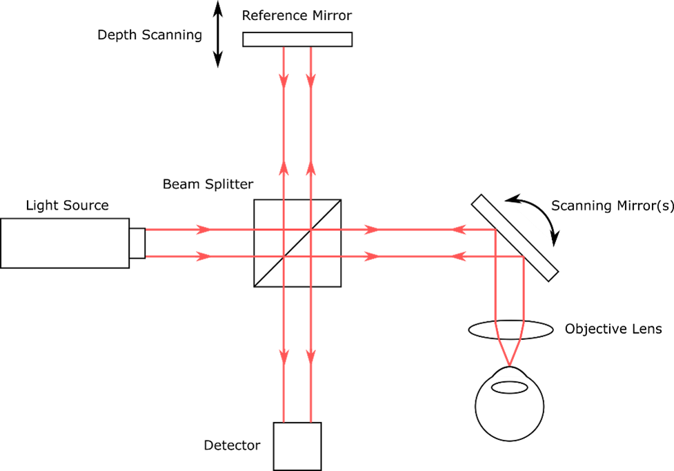Figure 3 A basic schematic of a single-point TD-OCT setup. Source; StarFish Medical.

Types of OCT

Several different techniques exist to collect the OCT signals needed to generate depth profiles.  These techniques can broadly be divided into “time-domain” and “frequency-domain” techniques.

In “time-domain” techniques (TD-OCT), the magnitude of light returning from different depths of the sample are inferred by changing the path length of the reference arm (or equivalently, the reference-arm light’s time of flight) and measuring the interference between the sample and reference light for each depth.

In “frequency-domain” techniques (FD-OCT), the spectrum of the recombined sample and reference light is measured with the reference arm at a fixed length. Interference between light from the two arms manifests as “fringes” in the measured spectrum. The time at which signals from different depths in the sample arrive at the detector and their magnitudes can be inferred from the measured spectrum using a Fourier transform, which mathematically describes a time-varying signal (in this case, light returning from the sample at various depths) as a function of its spectral amplitudes and phases.

Frequency-domain techniques can be further subdivided into “Spectral-domain” OCT (SD-OCT) and “Swept-source” OCT (SS-OCT).

In SD-OCT, a broadband light source is used to illuminate the sample.  After recombination of the sample and reference arms, the spectrum of the returned light is measured by dispersing the light onto a line detector (such as in a spectrometer).  The depth profile is then obtained via a Fourier transform of the spectrum. As all the information required to generate a depth scan is contained in the measured spectrum, depth scans can be captured at the frame rate of the line sensor.

In contrast, SS-OCT uses a “swept-source” laser with a narrow bandwidth whose center wavelength is repeatedly swept over a range of wavelengths, at sweep frequencies up to hundreds of thousands of times per second. By measuring the interference signal of the recombined light at each individual frequency, the full spectrum can be measured once every time the laser is swept.  Depth scans can then be calculated similarly as in SD-OCT.

OCT Imaging Techniques

Each of the modalities discussed above can be used with several imaging techniques for generating cross-sectional or 3D volumetric scans of the tissue under study.

In the most common approach, a focused point of laser light is rapidly scanned over the tissue to be investigated (sometimes called “single-point OCT”).  At each point where the laser is aimed, a depth profile is generated.  A lateral cross-section or 3D scan can then be generated by measuring the depth profile at many adjacent points.

Another imaging technique, called “line-field OCT”, simultaneously measures depth profiles from many adjacent points in a line, such that all the data required to generate a cross-sectional image are collected at the same time. This can be accomplished by using a line-scan sensor (essentially a 1D camera sensor) to receive the recombined light from multiple adjacent sample points on the adjacent pixels of the sensor.  The interference signals from each of the adjacent locations are then simultaneously generated by either moving the reference mirror (for TD-OCT), or by sweeping the wavelengths of the source (for SS-OCT). The corresponding depth profiles are generated from the frames captured on the line-scan sensor during the mirror movement/wavelength sweep.

Line-field OCT can also be used with SD-OCT using a slightly different method.  In that case, a 2D camera sensor is used.  Similarly to TD-OCT and SD-OCT line-field OCT, adjacent pixels on one axis of the sensor receive recombined light from adjacent points on the sample. On the second axis of the detector, a dispersive optic (such as a grating or a prism) is used along with appropriate imaging optics to spread out the light into its constituent wavelengths, thereby allowing the spectra from each adjacent point to be measured.  An advantage of this method is that each individual camera frame contains all the information required to produce a lateral cross-sectional image from the sample, with no need to move a mirror or sweep a wavelength source.

Finally, full-field OCT is an imaging technique that allows for simultaneous collection of depth profiles over many adjacent points in a 2D area, thereby allowing all the data required to generate a 3D volumetric scan to be collected at the same time. Similar to the (non-SD-OCT) line-scan method, recombined light from many adjacent points over a 2D area of the sample is imaged onto corresponding adjacent pixels on the detector.  By moving the reference mirror/sweeping the wavelength source, depth profiles for all the points in the area are collected, which are then combined to make a 3D dataset. Full-field OCT is generally not amenable to SD-OCT, as the spectrum of each point in the 2D area investigated cannot be simultaneously measured in a straightforward way, although novel approaches may overcome this limitation.

Advantages and Disadvantages of Different Types of OCT

Each of the types of OCT discussed can be useful in various contexts, and each have their own set of advantages and disadvantages. Some of the pros and cons of each of the techniques are summarized in table 1.  Note that the following discussion relates to typical approaches to OCT and may not apply to more novel approaches.

TD-OCT is the simplest technique conceptually. It is typically less expensive to implement than frequency domain techniques. It also has the longest possible imaging depth, limited only by the smaller of the distance the reference mirror can move and the depth into the sample from which measurable incident light is returned.  Furthermore, the sensitivity (i.e. limit of detectability) to a given amount of returned light is independent of the depth in the sample at which the light originated, which is not the case in SD-OCT (assuming the reference mirror is not moved). On the other hand, it can be shown that TD-OCT has the lowest overall signal-to-noise ratio of the modalities discussed (assuming shot noise limited detection) [4].  TD-OCT also has the slowest imaging rate (in terms of the rate at which A-scans can be collected) due to the required motion of the reference mirror, though this can be mitigated somewhat using line-field and full-field imaging techniques.

SD-OCT is generally capable of acquiring A-scans at a much faster rate than TD-OCT, limited by the readout rate of the sensor used to measure the spectrum (which can be up to hundreds of KHz).  SD-OCT also has a greater signal-to-noise ratio than TD-OCT, by a factor proportional to the number of pixels on the spectral detector used (again assuming shot noise limited detection) [4]. SD-OCT setups generally have the least complex detection scheme, as synchronization of the detection with the motion of the reference mirror/wavelength sweep is not necessary.

SD-OCT is likely to be more expensive to implement than TD-OCT, though the increase in cost can be relatively modest (driven primarily by the cost of the spectral detector). On the downside, the sensitivity of SD-OCT decreases as the path length difference between the fixed-length reference arm and the sample arm at a given depth increases (in contrast to TD-OCT which has a constant sensitivity with depth, owing to the motion of the reference mirror).  This limits the possible imaging depth of SD-OCT (unless the reference mirror is moved), which is inversely proportional to the spectral resolution of the detector.  Finally, SD-OCT cannot be straightforwardly implemented in a full-field setup, which limits the A-scan rate that may be achievable using that method.

SS-OCT is capable of acquiring A-scans even faster than SD-OCT, as the brightness of the source generally reduces the required exposure times per point, and because data from the detection electronics (usually photodiodes) can be read out at a faster rate.  SS-OCT has the same signal-to-noise ratio increase compared to TD-OCT as SD-OCT (with the increase in sensitivity being proportional to the number of sampled wavelengths from the swept source, rather than the number of pixels in a spectral detector).  SS-OCT can also be used with both line-field and full-field imaging.

While SS-OCT suffers from sensitivity decreases at increased reference/sample path length differences as in the case of SD-OCT, this disadvantage can be mitigated by the very narrow instantaneous linewidths and very small wavelength sweep step sizes that can be achieved with swept laser sources (corresponding to very high spectral resolution). Imaging depths >10 mm have been demonstrated in the human eye [5].

SS-OCT also has some downsides.  It is generally the most expensive type of OCT due to the high cost of the laser source and the high-speed electronics required.  The detection and triggering scheme required is also significantly more complex compared to that required for SD-OCT (and comparable to that required for TD-OCT).

In general, the best approach for a given OCT application will depend on the needs of the device under development.  Low-fidelity, low-cost approaches may be sufficient in some cases, whereas other approaches may require very high imaging speeds and high-fidelity results. Some applications may require only single depth scans or lateral cross-sections, whereas others may require full 3D volumetric data. Both the cost of the device and the quality of the OCT scans can be greatly affected by the OCT method used.

Table 1: Advantages and Disadvantages of Different Types of OCT. Source: StarFish Medical.

Method	Advantages	Disadvantages
TD-OCT	· Longest possible imaging range (assuming sufficient returned light) and constant sensitivity with depth · Can be combined with full-field OCT · Least expensive	· Slowest A-scan rate (by a wide margin) · Lowest signal-to-noise ratio
SD-OCT	· Higher A-scan rate than TD-OCT · Higher signal-to-noise ratio than TD-OCT · Least complex · Moderate cost	· Maximum imaging range is generally smaller than TD- and SS-OCT (limited by spectral resolution of detector) · Cannot be combined with full-field OCT
SS-OCT	· Higher A-scan rate than both TD- and SD-OCT · Higher signal-to-noise ratio than TD-OCT · Can be combined with full-field OCT	· Shorter imaging range than TD-OCT (but can be long regardless) · Most expensive

Conclusion

OCT is a powerful tool in medicine that allows semi-transparent internal structures of the body to be imaged in 3D with submillimeter resolution. The technique is used extensively in ophthalmology and optometry, and has potential applications in many fields including dentistry, dermatology, and gastroenterology.

This blog provides an overview of various OCT detection and imaging schemes. Each of these techniques comes with its own set of advantages and disadvantages.  In some applications, low-fidelity, low-cost solutions may be suitable, whereas other applications require state-of-the-art light sources and detections schemes that drive up cost but can result in much higher data collection rates and imaging fidelities.  An assessment of the requirements for a given OCT application is necessary to determine the best OCT method for that application.

StarFish Medical has experience designing and developing a number of OCT medical devices. Our optics team enjoys challenging medical device projects. Click here if you would like a free 30-minute consultation.

Bibliography

[1]	N. Le et al., “Intraoral optical coherence tomography and angiography combined with autofluorescence for dental assessment,” Biomedical Optics Express, vol. 13, no. 6, pp. 3629-3646, 2022.
[2]	M. Mogensen, “OCT imaging of skin cancer and other dermatological diseases,” Journal of Biophotonics, vol. 2, no. 6-7, pp. 442-451, 2009.
[3]	T. S. Kirtane and M. S. Wagh, “Endoscopic Optical Coherence Tomography (OCT): Advances in Gastrointestinal Imaging,” Gastroenterology Research and Practice, vol. 2014, no. 376367, pp. 1-7, 2014.
[4]	J. A. Izatt and M. A. Choma, “Theory of Optical Coherence Tomography,” in Drexler, W., Fujimoto, J.G. (eds) Optical Coherence Tomography. Biological and Medical Physics, Biomedical Engineering., Berlin, Heidelberg, Springer, 2008.
[5]	S. Chen et al., “High speed, long range, deep penetration swept source OCT for structural and angiographic imaging of the anterior eye,” Scientific Reports, vol. 12, no. 992, 2022.

Ryan Field is an Optical Engineer at StarFish Medical. Ryan holds a PhD in Physics from the University of Toronto. As a post doctoral fellow, he worked on the development of high-power picosecond infrared laser systems for surgical applications as well as a spectrometer from home materials.



---

• SEO Powered Content & PR Distribution. Get Amplified Today.
• PlatoData.Network Vertical Generative Ai. Empower Yourself. Access Here.
• PlatoAiStream. Web3 Intelligence. Knowledge Amplified. Access Here.
• PlatoESG. Carbon, CleanTech, Energy, Environment, Solar, Waste Management. Access Here.
• PlatoHealth. Biotech and Clinical Trials Intelligence. Access Here.
• Source: https://starfishmedical.com/blog/optical-coherence-tomography-types/