Mechanical stimulation and electrophysiological monitoring at subcellular resolution reveals differential mechanosensation of neurons within networks – Nature Nanotechnology

Primary neuron culture preparation

The experimental protocols involving animal tissue harvesting were approved by the veterinary office of the Canton Basel-Stadt according to Swiss federal laws on animal welfare and were carried out in accordance with the approved guidelines. HD-MEA chips or glass coverslips were sterilized in 70% ethanol for 60 min and washed with sterile deionized water under laminar airflow. The electrode array or the coverslips were then treated with 10 µl of 0.05% (v/v) poly(ethyleneimine) (Sigma-Aldrich) in borate buffer (Thermo Fisher Scientific) for 40 min at room temperature and washed with deionized water, followed by incubation with 8 µl of 0.02 mg ml^–1 laminin (Sigma-Aldrich) in neurobasal (NB) medium (Gibco) for 30 min at 37 °C. E-18 Wistar rat embryos were dissected in ice-cold HBSS (Gibco) to harvest their cortices, which were then dissociated in 0.25% trypsin–EDTA (Gibco). The dissociated cortical cells were gently triturated and filtered through a 0.45 µm sieve to obtain single cells. Cell density was estimated, and 10 µl of 3,000 cells µl^–1 solution was plated on the electrode array. Cells were allowed to attach to the arrays by incubating the chips at 37 °C for 40 min before adding 2 ml of NB plating medium. NB plating medium was prepared by adding 50 ml horse serum (HyClone), 1.25 ml glutamax (Invitrogen) and 10 ml B-27 (Invitrogen) to 450 ml Neurobasal (Gibco). The HD-MEA chips were kept inside a cell culture incubator at 37 °C and 5% CO₂. After 3 days, the cells were cultured in serum-free NB plating medium up to DIV 20 by exchanging 50% of culture media with fresh NB plating medium once every 3 days. All experiments, except for the data shown in Fig. 1i, were conducted between DIV 14 and 16 because cells showed different mechanical properties while growing¹¹. The experiments for the data shown in Fig. 1i were collected between DIV 22 and 24, when the neuronal networks showed synchronous bursting activity.

Cerebellum slice preparation

Wild-type mice (postnatal day 14 C57BL/6Rj, Janvier Labs) were decapitated under isoflurane anaesthesia; their brains were removed and immersed into ice-cold carbogen-bubbled (95% O₂ + 5% CO₂) artificial cerebrospinal fluid (aCSF) solution. Sagittal cerebellar slices of ∼350 µm were obtained using a vibratome (VT1200S, Leica). All slices were maintained at room temperature in aCSF until use. The aCSF was composed of 125 mM NaCl, 2.5 mM KCl, 2 mM CaCl₂, 1 mM MgCl₂, 25 mM glucose, 1.25 mM NaH₂PO₄ and 25 mM NaHCO₃. The electrode array of the HD-MEA chips was then treated with 10 µl of 0.05% (v/v) poly(ethyleneimine) (Sigma-Aldrich) in borate buffer (Thermo Fisher Scientific) for 40 min at room temperature and washed with deionized water, followed by an incubation with 8 µl of 0.02 mg ml^–1 laminin (Sigma-Aldrich) in Neurobasal medium (Gibco) for 30 min at 37 °C. Excess laminin after incubation was pipetted out, and the array was allowed to dry. The cerebellar slice was then gently placed on the electrode array using a cut pipette tip to avoid damage caused by shear forces during pipetting (Supplementary Fig. 13). A 2 mm custom-made harp was placed on the tissue slice to immobilize the tissue slice. Tissue slices were then immersed in aCSF by gently adding drop by drop. The immobilized tissue slice immersed in aCSF was then allowed to adhere to the electrode array for 30 min. Just before the recording, the harp was removed, and the AFM head was mounted onto the HD-MEA chip. The tissue was continuously perfused with carbogen-bubbled aCSF to maintain cell viability and activity.

HD-MEA set-up

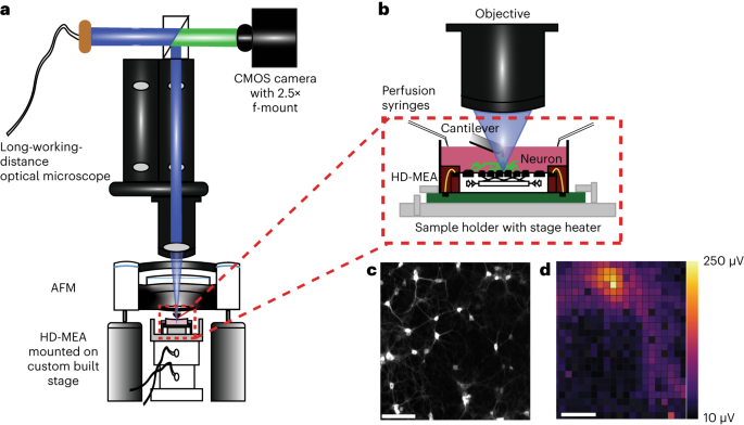
Complementary-metal-oxide-semiconductor (CMOS)-based HD-MEA chips featuring 26,400 electrodes (17.5 µm pitch) within an overall sensing area of 3.85 × 2.10 mm² were used²⁵. The chips were fabricated in a commercial foundry and post-processed and packaged in house (Supplementary Fig. 1b). Transparent polycarbonate rings (GB Plex) of 4 cm diameter were glued onto the chips, and the wire bonds were encapsulated with biocompatible dark epoxy (EPO-TEK 353 ND). The platinum-black coating of the electrodes was electrodeposited to decrease the electrode impedance and improve the signal-to-noise characteristics (Supplementary Fig. 1c). Commercial versions of our custom-developed HD-MEA system can be purchased (MaxOne model) from MaxWell Biosystems.

Sample holder and stage heater

A thermoelectric Peltier-based sample heater, with a temperature probe for closed-loop feedback, was controlled by a home-built temperature controller to maintain the sample at 37 °C. The sample heater was aligned with the thermal conduction pad on the HD-MEA chip. The chips were then mounted onto a sample holder and locked in position with the holder’s spring-loaded pin. Prusa I3 MK3S+ was used to 3D print the frugal syringe holders for the perfusion set-up which were attached to the sample holder. The entire set-up was mounted onto a custom-made x,y piezo stage via a base plate.

x,y piezo stage

Two linear piezo stages (Xeryon XLS-1 series) with an encoder resolution of 5 nm were attached to each other perpendicularly (Supplementary Fig. 1a). The linear stages were controlled by a Xeryon XD-M multiaxis controller connected to a LabVIEW-based user interface. The top left electrode of the HD-MEA chip was registered as the origin of the coordinate system, and the electrode coordinates with the neurons of interest were extracted from the MaxWell Biosystems user interface. These coordinates were then fed to the XD-M controller using custom scripts for easy positioning of neurons under the AFM cantilever.

Long-working-distance fluorescence microscopy

An optical microscope (Nikon SMZ 25) with 15.75× adjustable zooming lenses and 1× objective (Nikon, MNH55100 P2-SHR PlanApo 1X; numerical aperture, 0.156) was aligned with the set-up as mentioned in main text. A TTL-controllable light-emitting diode (LED) illuminator (CoolLED PE 300^ultra) was used as a light source for excitation/emission filter-free imaging. A triple bandpass beam splitter (F66-412, AHF Analysentechnik) was used to filter the reflected excitation light from the HD-MEA chip. A large CMOS array camera (Nikon DS-QI2) with 4,908 × 3,264 pixels (pixel size, 7.3 × 7.3 µm²) was mounted onto the microscope using a 2.5× f-mounted projector lens allowing for sampling of up to 45 f.p.s. with a final magnification of ∼40× and a resolution of 0.46 µm per pixel.

AFM

An AFM head (Catalyst, Bruker) was mounted and aligned with the set-up as mentioned in the main text. A 15 µm piezo scanner on the head was used to collect all force–displacement and force–time curves, while a 150 µm piezo was used to position the cantilever on the neuron. The data were collected and exported to .txt files using the AFM software (Nanoscope v.9.2, Bruker). The data were analysed and plotted with Python scripts. Silica beads with 5 μm diameter (Kisker Biotech) were glued to the free end of tipless microcantilevers (CSC-37 or 38, Micromash HQ) using ultraviolet glue (Dymax) and were ultraviolet cured for 20 min. Beaded cantilevers were cleaned for 5 min using a plasma cleaner (Harrick Plasma), then mounted onto the fluid probe holder with a 2 mm sapphire window, and calibrated using the thermal noise method⁴⁸.

Correlative AFM, HD-MEA and optical microscopy

The AFM, HD-MEA and optical microscope were aligned as shown (Fig. 1a). Fluorescence light from neurons on HD-MEA chips was collected through a sapphire window in the AFM cantilever holder and passed to the optical microscope. The fluorescence image of the neurons on the HD-MEA chip were sequentially collected in regions of interest, stitched and registered on the Maxwell MEA user interface to localize neurons on the HD-MEA chip (Supplementary Fig. 2a–d). The x,y coordinates of neurons of interest were then fed to the x,y stage via LabVIEW scripts, thus placing the AFM cantilever at the desired positions with ∼5 nm precision. The entire set-up was installed on a damping isolated table and placed in a noise-protected, temperature-controlled chamber to reduce mechanical noise and thermal drift.

TTL synchronization

TTL pulses from DS-Qi2 were extracted using a home-built connector with a 3.5 inch four-pole pin, a mini plug on one side and a female 24 AWG jumper (RND 255-00015, Distrelec) on the other side. Pin 1 was the ground and pin 4 (EXP_TMG) received 2.4 V on HI (high) level at live operation according to the set exposure time. A negative pulse of 0–5 V was extracted from the front panel output channel 1 of the AFM controller (Bruker Nanoscope V) through a home-built connector with a standard BNC male pin on one side and a female 24 AWG jumper (RND 255-00015, Distrelec) on the other side. The signals, extracted from both camera and AFM, were then routed to pin 2 and 8 of a single high-speed optocoupler. The signals were then sent to the HD-MEA data-acquisition system via a field-programmable gate array, providing precise time stamps of the events detected by AFM and optical microscopy on raw file recordings of HD-MEA data collected at 20 kHz.

Stiffness tracking protocol and measurements

The apparent Young’s modulus was calculated from an average of five force–displacement curves collected on the neuronal soma. We then waited for 30 s to ensure that there were no measurement-induced mechanical changes in the neurons and collected five force–displacement curves again (Fig. 2a), which we labelled as one measurement cycle and which is represented by one dot (Fig. 2b). We repeated this measurement cycle up to 5 min on a neuron and moved to the next neuron in the network. Sixty minutes after the first measurement on the first neuron, we returned to the same neuron, and the measurement cycle was repeated. The measurements comprised a long-time-scale-tracking cycle. This long-time-scale tracking cycle was repeated three times (Fig. 2c). For stiffness measurements of neurites, we first recorded the electrophysiological activity of the neurons for 5 min and then identified two well-isolated neurites per neuron and collected force–displacement curves on them. Force–displacement curves were collected using CSC-38 microcantilevers (nominal spring constant, ∼0.02 N m^–1) featuring 5-μm-diameter beads as mentioned above. A maximal force of 700 pN on somas and of 400 pN on neurites was used to collect force–distance curves (Supplementary Fig. 14a,b). For all the measurements, the tip velocity was kept constant at 10 µm s^–1. The contact point was determined from the approach force–displacement curve as the x intercept at a value of force, which was five times higher than the standard deviation of baseline noise, followed by a manual curation. Indentation depth was calculated as the displacement value at the contact point after subtracting the cantilever deflection and setting the displacement value at the maximal force to zero in the force–displacement curve (Supplementary Fig. 14c). The indentation depth for the same given maximal force would vary from soma to soma depending on its stiffness. Therefore, we have set an indentation depth cut-off of 750 nm. In the force–displacement curves, all force values for which the corresponding displacement value exceeded the indentation depth cut-off were discarded. The apparent Young’s modulus was calculated from such curves to which the Hertz model for a spherical indenter with an elastic half-space⁴⁹ was fitted using custom codes in Python.

The Young’s modulus values measured in our study for the soma of neurons are in a comparable range with previous reports^10,11. However, the Young’s modulus of the neurites is lower than the reported values, while they still are on a comparable order of magnitude. This bias might result from our choice to measure the two thickest basal neurites of the neuron, which are typically softer. For measuring the stiffness of the neuronal somas during burst and IBIs, we have collected force–displacement curves at a frequency of 5 Hz. This process was repeated several times for each soma, and the average stiffness of the soma during bursting periods and during IBIs was calculated. While the bursts usually appear in a rhythmic pattern (Fig. 2h), it is difficult to predict for cultured neurons when a single neuron undergoes bursting. To collect at least two force–displacement curves during bursting periods or IBIs, while minimizing the number of times the probe comes in contact with the neuron, we indented the neuron 5 times s⁻¹.

Static compression protocol

A 5-µm-diameter bead, glued to a tipless AFM microcantilever (CSC-37; nominal spring constant, ∼0.8 N m^–1), was positioned above the soma. The bead was lowered onto the soma until a setpoint force required to apply 0.1 kPa or 5 kPa was reached and kept in contact for 60 s using constant-height feedback before retracting the bead (Fig. 5b). The force–time curve recorded at 500 kHz sampling rate shows both the vertical displacement of the AFM head and the force response of the soma. The average height of soma of rat cortical neurons was ∼8 µm (Supplementary Fig. 11a).

Functional calcium imaging

Genetically encoded calcium sensors were expressed in neurons using adeno-associated viruses (AAVs). AAV1-EF1a-GCaMP6s (1.8 × 10¹³ viral genomes ml⁻¹) were used at a multiplicity of infections of 5.0 × 10⁴ to express GCaMP6s. Neurons were infected at DIV 3; expression was usually seen at DIV 5–9.

Functional calcium imaging analysis of mechanically stimulated neurons

An average fluorescence intensity curve ΔI/I of the GCaMP6s curve was calculated as the mean signal over the entire image relative to the baseline of the image. Peak detection in the signal was performed by finding local maxima within a 3 s window. An event was marked as the start of a neuronal response when the calcium signal amplitude reached 10% of the peak value. Data from 2.5 s before and 10 s after the start of the response peak (t = 0) was plotted.

HD-MEA recordings

The MaxWell Biosystem user interface (MaxLab Live v.22.13) was used to record the data. The whole-chip fluorescence image was registered on the user interface (Supplementary Fig. 2c). Neurons of interest were identified from calcium spikes, and spiking activity (action potentials) was obtained from the live raster plots on the user interface. Once a neuron of interest was identified, 512 electrodes around this neuron in a rectangular configuration were routed to the readout. After positioning the AFM cantilever on the neuron, the channels were offset five times to compensate the noise from the infrared laser used by the AFM to detect the cantilever deflection before starting the recording. A gain of 512 and a high-pass filter with a cut-off at 300 Hz were used for all recordings. To improve the performance of the spike-sorting algorithms in Fig. 5, neuronal action potentials were recorded 2.5 min before and after mechanical stimulation.

HD-MEA data analysis

All collected HD-MEA data were processed via custom scripts based on Spikeinterface⁵⁰. Briefly, extracellular recordings were filtered and spike-sorted using Kilosort2, followed by manual curation of all recordings. A conservative inter-spike interval violation threshold of 0.5 and a signal-to-noise ratio threshold of 5.0 were used for curation. Template similarity, auto-correlograms and cross-correlograms were used for unit quality assessment. Waveform features such as halfwidth and repolarization slope were extracted for spike-sorted units for the respective epochs with Python scripts using functions from Spikeinterface (Supplementary Fig. 12a–i). The relative changes in the waveform features on all electrodes within the extracellular footprint of a neuron were obtained by dividing the value of the mean waveform feature of all spikes during mechanical compression by the mean waveform feature of all spikes before compression. Mean firing rate and inter-spike interval were computed from the extracted spike trains using the Elephant electrophysiology analysis toolkit 0.11.2⁵¹. The mean firing rates for stiffness correlation data were computed by placing the spikes in 30 s bins to match with the time points of the stiffness values. The mean firing rates for the compression protocol were computed by placing spikes in three bins of before, during and after compression.

Combined AFM and confocal microscopy

Time-lapse confocal imaging was performed on an inverted laser-scanning confocal microscope (Observer Z1, LSM 700; Zeiss) equipped with a 25×/0.8 LCI PlanApo water immersion objective (Zeiss). An AFM (CellHesion 200; JPK Instruments) was mounted onto the confocal microscope. Mechanical compression protocols were executed using JPK CellHesion software. For mechanical stimulation, AFM was used to approach the cantilever with the bead onto the cell at speeds of 0.1, 1, 10 or 100 μm s^–1 until reaching the setpoint force, and, thereafter, immediately retracted at the same speed as used for the approach. For experiments determining the threshold force to mechanically stimulate neurons, the applied setpoint force was stepwise increased from 50 to 400 nN in 50 nN increments and intervals of 20 s (Supplementary Fig. 6). The setpoint force of the approaching bead was stepwise increased until a neuronal response was recorded. After successful stimulation of the neuron, the cantilever was retracted, and a new neuron was selected for stimulation.

Statistical analysis

All data showing waveform properties were tested for normality with the Shapiro–Wilk test and Q–Q plots. All data groups were not normally distributed and were dependent data groups. Therefore, we used the Wilcoxon signed-rank test. The null hypothesis was that there is no difference in medians between the pairwise compared distributions. P values >0.05 were considered non-significant. The waveform features were extracted from the averaged waveform of each neuron obtained from n > 5,000 spikes. All data showing mean firing rates were compared with the Wilcoxon signed-rank test from n > 10,000 spikes. AFM data groups were compared using the two-tailed Mann–Whitney U-test. P values for each comparison are mentioned in the figure legends. Pearson correlation was used to determine the linear correlations in stiffness and mean firing rate values. No statistical methods were used to predetermine sample sizes. Data collection and analysis were not performed blind to the conditions of the experiments.

Reporting summary

Further information on research design is available in the Nature Portfolio Reporting Summary linked to this article.

• SEO Powered Content & PR Distribution. Get Amplified Today.
• PlatoData.Network Vertical Generative Ai. Empower Yourself. Access Here.
• PlatoAiStream. Web3 Intelligence. Knowledge Amplified. Access Here.
• PlatoESG. Carbon, CleanTech, Energy, Environment, Solar, Waste Management. Access Here.
• PlatoHealth. Biotech and Clinical Trials Intelligence. Access Here.
• Source: https://www.nature.com/articles/s41565-024-01609-1